What is CoRA?
Commingled human remains are often encountered in archaeological and forensic contexts. A bone by bone inventory is an important step in segregating commingled remains into individuals and determining the minimum number of individuals present. In order to achieve individual identification a controlled and consistent specimen-level inventory procedure must be followed. The Commingled Remains Analytics (CoRA) web application, database and APIs are a community resource for inventorying assemblages of commingled human remains, while providing a framework of analytic methods, visualization techniques and tools to assist in the segregation and identification process.
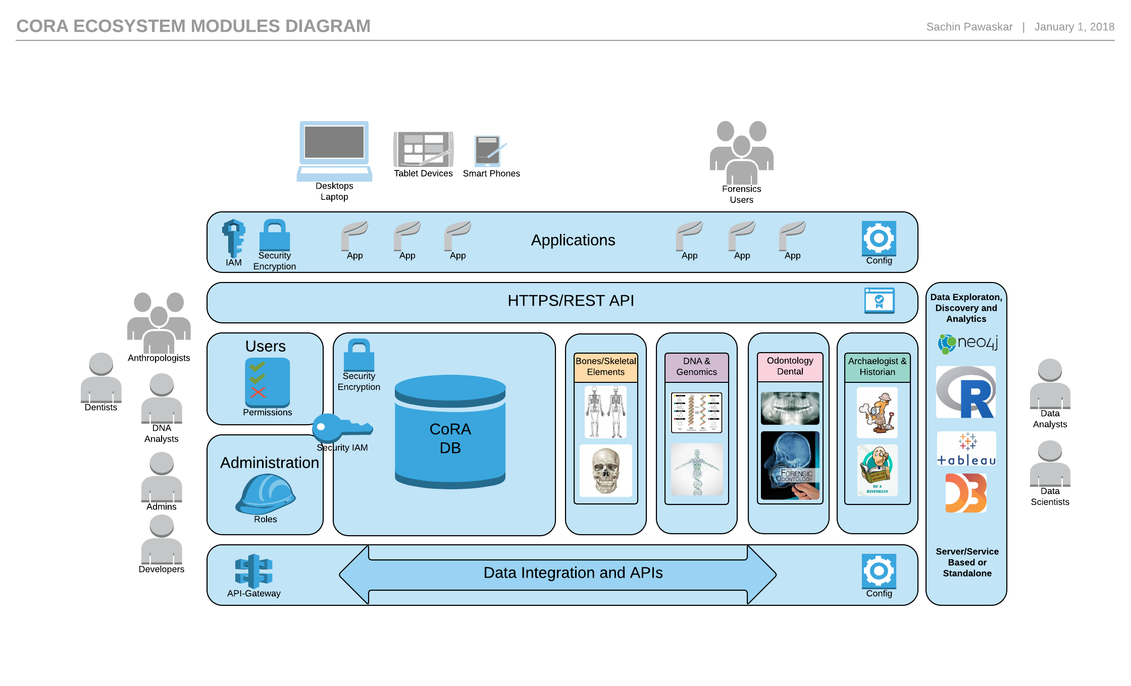
CoRA Ecosystem
The CoRA Ecosystem is built on a flexible, extensible and modular architecture, allowing for new modules to be added. It provides for easy integration with the flexibility to add new applications based on the cora data and integration frameworks. Users will be able to easily access their data via the data integration API allowing for integrations with other external systems as well as use for advanced analytics modules based upon new research, tools and technologies.
Security
The CoRA Ecosystem is built with security in mind. The CoRA application and information systems meets the minimum requirements as outlined in the DoDI 8582.01 and NIST SP 800-171-r2 the authoritative source of the CUI security requirements. The security requirements in SP 800-171 Revision 2 are available in multiple data formats and are available to download at NIST SP 800-171.
In the near future, we plan to be in compliance with the Cybersecurity Maturity Model Certification (CMMC) which is a unifying standard for the implementation of cybersecurity across the Defense Industrial Base (DIB). The CMMC framework includes a comprehensive and scalable certification element to verify the implementation of processes and practices associated with the achievement of a cybersecurity maturity level. The CMMC 2.0 Model is designed to provide increased assurance to the Department that a DIB company can adequately protect sensitive unclassified information, accounting for information flow down to subcontractors in a multi-tier supply chain.
How do I report a security vulnerability?
If you discover a security vulnerability within CoRA, please create an issue on GitHub or please send an e-mail to Sachin Pawaskar at sachinpawaskar@msn.com or spawaskar@unomaha.edu. All security vulnerabilities will be promptly addressed.
Contribution Guidelines
If you are submitting documentation for the current stable release, submit it to the corresponding branch. For example, documentation for CoRA 1.0 would be submitted to the 1.0 branch, documentation for CoRA 2.0 would be submitted to the 2.0 branch and so on. Documentation intended for the next release of CoRA should be submitted to the master branch.
How to Cite CoRA?
How do I Cite CoRA?
(Pawaskar et al., 2021)
(Pawaskar et al., 2021) as

Sachin Pawaskar, E. Streetman, C. LeGarde, N. Jensen, S. Raut, F. Damann, V. Rahangdale, J. Smith, W. Wetzel, C. Venkatesan, L. Biehler-Gomez, K. East, T. V. Deest, J. Lynch, b. New, & Sihley Pawaskar. (2021). spawaskar-cora/cora-docs: Open Community Release (v2.1.0). Zenodo. https://doi.org/10.5281/zenodo.5694496
Getting started
Getting started
Congratulations you have found the CoRA User guide. This manual is intended to help you get the most out of your CoRA application in your day-to-day use.
This guide answers the “why, where, and how” questions that most users have when learning to use the CoRA platform. You’ll find lots of step-by-step instructions, screenshots, and examples. You’ll get an overview of the modules & resources that are available to you as you work on your Forensic Anthropology projects in CoRA. Finally, you’ll learn the concepts of the CoRA platform with it powerful configuration features, and establish best practices for project standards and requirements.
Tip
CoRA can be used for inventorying assemblages of single or commingled human remains
Commingled human remains are often encountered in archaeological and forensic contexts. A bone by bone inventory is an important step in segregating commingled remains into individuals and determining the minimum number of individuals present. In order to achieve individual identification a controlled and consistent specimen-level inventory procedure must be followed.
The Commingled Remains Analytics (CoRA)1 web application, database and APIs are a powerful community resource for inventorying assemblages of single or commingled human remains, while providing a framework of analytic methods, visualization techniques and tools to assist in the segregation and identification process.
(CoRA)1 is a powerful web application ecosystem with an open, flexible, scalable, plug-n-play architecture and framework.
Installation
If you are wondering what you need to install to start using CoRA for your forensic anthropology project, the answer is NOTHING Yes I know its hard to believe, but its true CoRA is built and deployed as a Software as a Service (Saas) model. Why? you ask, because we believe that you should focus on what you are good at and leave the mundane technical software and hardware stuff to us.
How do I get started
To get started with CoRA you can reach out to the author Dr. Sachin Pawaskar on this personal email sachinpawaskar@msn.com or his university email spawaskar@unomaha.edu with information about who you are? what is the project that you want to use CoRA for? who are you affiliated with? to start off with. Dr. Pawaskar with get back to you to get started the process of using CoRA for your project.
Organizations, Users and Projects
To keep your data secure and organized, the CoRA application is structured around the concept of organizations, users and projects. So, What does this mean for you? Well, it means your organization data is secured and no one from another organization can access your data, Only users within your organization can access your data. Data is typically organized by projects and only those users within your organization who have access to the project are allowed to access your project specific data.
CoRA was designed to be used by both organizations and single users. Organizations can be government organizations, non-profits, universities or any entity that deals with the identification of missing persons, or segregation of human remains. Single users could be any single individual who wants to use CoRA for their own project, a use case might be for university students of forensic anthropology for their Dissertation, Thesis, Independent Study or Graduate Project work.
Sample Graduate Student Thesis
Madeline Grace Kelly used CoRA for her graduate thesis work at Syracuse University. Her research work is titled Analysis and Quantification of Commingled Human Skeletal Remains in Syracuse University. Here is her graduate thesis work and her thesis presentation. You can reach out to Madeline to hear more about her experience with CoRA.
Who might benefit from the use of CoRA?
CoRA was designed to be used by both government agencies, universities and single users such as students.
- Organizations can be government organizations, both federal and local governments or law enforcement.
- Non-profits organizations whose mission is to seek social justice for those missing.
- Universities who have any medical exemplars of human remains for teaching purposes.
- Students or Individual users who wants to use CoRA for their own project, a use case might be for university students of forensic anthropology for their Dissertation, Thesis, Independent Study or Graduate Project Work.
- Any entity that deals with the identification of missing persons, or segregation of human remains.
Reach out over email
You can reach out to to the author Dr. Sachin Pawaskar on his personal email sachinpawaskar@msn.com or his university spawaskar@unomaha.edu.
Initial Setup Template
Once we establish the usage of CoRA for your organization or project, you will have to provide some initial setup information related to the organization, project and its users by filling out the following cora new organization projects and users template
Fill out an issue template
On Github
-
In 2016, CoRA started out as a simple specimen inventory system for Forensic Anthropologists. It was first showcased at the AAFS 70th Annual Conference in Seattle, WA in February 2018, but over the course of several years, it's now much more than that – with the many built-in modules such as specimens, dnas, dental, isotopes, missing persons, dashboards, reports, search, analytics, visualizations, administration, projects, user settings, and countless customization abilities. CoRA is now one of the simplest and most powerful frameworks for managing a single individual remains project or a complex commingled remains project. ↩↩
Philosophy
Before settling for CoRA, it's a good idea to understand the philosophy behind the CoRA Ecosystem, in order to make sure it aligns with your goals and project needs. This page explains the design principles anchored in CoRA and explains them briefly in this documentation.
Design principles
 It's a Saas Web Application
Focus on the forensic anthropology skills you are good at and leave the software and hardware issues to us, because CoRA is managed as Software as a service (Saas). No need to know Programming, Databases, HTML, CSS or JavaScript.
- Let CoRA do the heavy lifting for you.
Advanced Analytics & Visualizations
Provides the most advanced, current and modern analytics and visualizations to help you find things that matter using state-of-the-art algorithms including advanced statistical techniques & regression models, graph theory and AI/ML models.
– The algorithms in CoRA are designed to help you find things that matter
Works on all devices
Serve your project needs with confidence – the underlying layout, screens, widgets, styles and user interface automatically adapts to perfectly fit the available screen real estate, no matter the type or size of the viewing device.
– CoRA works where you are, on any device
Made to measure
Change the colors, notifications, org, project & user settings and much more with just a few clicks. CoRA can be easily customized and provides tons of options to alter appearance and behavior.
– CoRA is a delight to work with.
Fast and lightweight
Don't let your users wait – get incredible value with a small footprint, by using one of the fastest specimen inventorying system around with excellent performance and traceability resulting in faster and accurate identifications.
– CoRA delivers on a consistent basis
Accessible
Make accessibility a priority – users can navigate your project data with touch devices, keyboard, and screen readers. Semantic ARIA support ensures that CoRA works for everyone.
– CoRA is crafted for all, no one left behind
Open Community Driven
Trust users across the globe – choose a mature solution built with state-of-the-art Open Source technologies. Keep ownership of your content without fear of data lock-in.
– CoRA is build by people like you
Conventions
This section explains several conventions used in CoRA and this documentation.
How can I add a new or missing convention symbol to CoRA?
You can request new or missing convention symbol to be added to CoRA if the one you are looking for is not present by creating an issue on our issue tracker.
Symbols
This CoRA application and documentation uses some symbols for illustration purposes. Knowing what these symbols are and what they denote will help you to navigate in CoRA. Before you read on, please make sure you've made yourself familiar with the following list of conventions:
– Specimen
The skull symbol denotes that the Specimen module is available to the user. Make sure you have the necessary permissions to use the specimen module and its features.
- DNA
The dna symbol denotes that the DNA module is available to the user. Make sure you have the necessary permissions to use the dna module and its features.
– Isotope
The isotope or radioactive symbol denotes that the Isotope module is available to the user. Make sure you have the necessary permissions to use the isotope module and its features.
– Dental
The tooth symbol denotes that the Dental module is available to the user. Make sure you have the necessary permissions to use the dental module and its features.
– Individual
The individual symbol denotes that the Individual module is available to the user. Make sure you have the necessary permissions to use the individual module and its features.
– Missing Person
The missing persons symbol denotes that the Missing persons module is available to the user. Make sure you have the necessary permissions to use the missing persons module and its features.
- DNA sampled
The DNA symbol in conjunction with a green ✔ check mark denotes that a specimen has been DNA sampled. A number next to the check mark denotes the mito sequence number associated with it. The DNA symbol in conjunction with a red ❌ cross mark denotes that a specimen has not been DNA sampled yet.
– Isotope sampled
The Isotope symbol in conjunction with a green ✔ check mark denotes that a specimen has been Isotope sampled. The Isotope symbol in conjunction with a red ❌ cross mark denotes that a specimen has not been Isotope sampled yet.
– Measurements
The Measurements symbol in conjunction with a green ✔ check mark denotes that a specimen has been measured. The Measurements symbol in conjunction with a red ❌ cross mark denotes that a specimen has not been measured yet.
– Zones
The Zones symbol in conjunction with a green ✔ check mark denotes that a specimen has zonal classification done. The Zones symbol in conjunction with a red ❌ cross mark denotes that a specimen has not had zonal classification done yet.
– XRay
The XRay symbol in conjunction with a green ✔ check mark denotes that a specimen has been XRayed. The XRay symbol in conjunction with a red ❌ cross mark denotes that a specimen has not been XRayed yet.
– CT Scanned
The CT Scanned symbol in conjunction with a green ✔ check mark denotes that a specimen has been CT Scanned. The CT Scanned symbol in conjunction with a red ❌ cross mark denotes that a specimen has not been CT Scanned yet.
– Inventoried
The Inventoried symbol in conjunction with a green ✔ check mark denotes that a specimen has inventory completed. The Inventoried symbol in conjunction with a red ❌ cross mark denotes that a specimen has not been inventory completed yet.
– Reviewed
The Reviewed symbol in conjunction with a green ✔ check mark denotes that a specimen has been reviewed. The Reviewed symbol in conjunction with a red ❌ cross mark denotes that a specimen has not been reviewed yet.
– Help
The Help symbol denotes that there is a help page for the specific screen the user is currently viewing. Clicking the help link will take you to the relevant help page on https://doc.coracore.org
– Search
The Search symbol denotes that you can perform a search on a specific page. There is a global search bar available that allows the user to search the specimens, dnas, isotopes, dental, individuals and missing persons models which will return a data table of all records within the current project that match the search criteria.
– Search History
The Search history symbol denotes that you can save or favorite your most frequently used searches. This feature allows users to re-run previously searched models within a project. The Search history has two parts, the search history part shows the last 10 searches the user has performed and the search favorites which allows the user to favorite and run a previous search done by the user. This ia a very powerful and useful capability that is liked by most users.
– Notification
The Notification symbol denotes that you have notifications. A number badge next to the notification symbol denotes the number of unread notifications or messages.
– Full Window
The Full Window symbol allows the user to maximize the current page or screen the user is viewing. Clicking this symbol will expand the current screen by full size by removing the browser title, address and button bars while maximizing the browser window to create more screen real estate.
– Dashboard
The Dashboard symbol allows the user to view the dashboard page. Depending on the user privileges either the Org, Project or User dashboard will be made available to the user. The dashboard itself contains many widgets which show various charts and numbers relevant to the org, project or user.
– Biological Profile
The male/female symbol denotes that the biological profile for a specimen. The biological profile is available under more actions button on the specimen screens if that specimen bone has any methods associated with it such as age, sex, ancestry and stature.
– Age
The number or pound symbol denotes that age methods for a specimen. The age methods are available in the biological profile menu under more actions button on the specimen screens if that specimen bone has any associated age methods.
– Sex
The human male/female symbol denotes that sex methods for a specimen. The sex methods are available in the biological profile menu under more actions button on the specimen screens if that specimen bone has any associated sex methods.
– Ancestry
The leaf symbol denotes that ancestry methods for a specimen. The ancestry methods are available in the biological profile menu under more actions button on the specimen screens if that specimen bone has any associated ancestry methods.
– Stature
The human height symbol denotes that stature methods for a specimen. The stature methods are available in the biological profile menu under more actions button on the specimen screens if that specimen bone has any associated stature methods.
– Taphonomy
The "T" symbol denotes that taphonomies can be associated with a specimen. The taphonomies are available under more actions button on the specimen screens.
– Measurements
The square ruler symbol denotes that measurements can be associated with a specimen. The measurements are available under more actions button on the specimen screens if that specimen bone has allowed measurements.
– Zone Classification
The group symbol denotes that zonal classifications can be associated with a specimen. The zonal classification are available under more actions button on the specimen screens if that specimen bone has allowed zonal classification.
– Associations
The link ruler symbol denotes that associations can be made for a specimen. The associations is available under more actions button on the specimen screens if that specimen bone has any associations allowed such as articulations, pair match, refits and morphology. Typically one specimen is related or associated with another specimen via the articulation, pair match, refit or morphology relationship
– Articulations
The chain link symbol denotes that articulation are allowed for a specimen. The articulations are available in the associations menu under more actions button on the specimen screens if that specimen bone is articulated with other bones.
– Pair Matching
The left-right symbol denotes that pair matching are allowed for a specimen. The pair matching are available in the associations menu under more actions button on the specimen screens if that specimen bone is a paired bone meaning that it can be a left and right sided bone.
– Refits
The puzzle symbol denotes that refits are allowed for a specimen. The refits are available in the associations menu under more actions button on the specimen screens if that specimen bone has a refit flag. Typically most bones can be refit.
– Morphology
The shape symbol denotes that morphology associations are allowed for a specimen. The morphology are available in the associations menu under more actions button on the specimen screens if that specimen bone has a morphology flag. Typically most bones can be morphologically associated.
– Pathology
The flask symbol denotes that pathologies can be assigned for a specimen. The pathologies are available in the pathology menu under more actions button on the specimen screens.
– Trauma
The gun symbol denotes that traumas can be assigned for a specimen. The trauma are available in the pathology menu under more actions button on the specimen screens.
– Anomaly
The lightening symbol denotes that anomalies can be assigned for a specimen. The anomalies are available in the pathology menu under more actions button on the specimen screens if that specimen bone has anomalies for that bone.
– Review
The eye symbol denotes that a review can be performed for a specimen. The review menu is available under more actions button on the specimen screens.
– Tag
The tag symbol denotes that tags have been assigned for a model (such as specimens, dna, etc). The user can assign multiple tags to a specimen. Tagging is a simple way of grouping, marking or flagging a specimen for further action in the future. Think about tagging as a way collecting, bagging or grouping specimens. It is a powerful feature in CoRA for segregation and analysis purposes.
– Comment
The comment symbol denotes that tags have been assigned for a model (such as specimens, dna, etc). The user can assign multiple comments to a specimen. Comments are useful to provide additional information to the forensic scientist or project team for possible insights in the future. It can also be used by the project team to communicate additional information about a specimen.
– File
The files symbol denotes that the File module is available to the user. Make sure you have the necessary permissions to use the file module and its features which include file export, import and search.
– File Export
The file export symbol denotes that the File export feature is available to the user. Make sure you have the necessary permissions to use the file export feature.
– File Import
The file import symbol denotes that the File import feature is available to the user. Make sure you have the necessary permissions to use the file import feature.
– File Search
The file search symbol denotes that the File search/manage feature is available to the user. Make sure you have the necessary permissions to use the file search/manage feature.
– Analytics
The graph symbol denotes that the analytics and visualization feature is available to the user. Make sure you have the necessary permissions to use the analytics and visualization feature.
Customization
Warning
This page is work in progress.
CoRA was built from the ground up you the user, front and center in mind. CoRA allows for customization at the Org, Project and User levels. Each users can customize their own user expereince. We recognize that each one of you is a unique individual with differing ways of working with your project data. Moreover each project has different and unique needs and requirements, hence customizing at the project level is a must. Finally customizations are available at the organization level allowing org administrators to enforce guidelines and standards.
User
Project
Org
Enterprise Feedback
Warning
This page is work in progress.
We highly value the insights of our enterprise users, and we're eager to hear from you. Your feedback is immensely valuable to us. If you're utilizing CoRA in an enterprise context and would like to share your experiences with us, we'd love to connect and discuss:
- What you are building with it
- What aspects you like about it
- What challenges you are facing
- What could be improved
Let's Connect
To schedule a convenient appointment, please reach out to us via email at sachinpawaskar@msn.com and provide us with the following details:
- Your company's name
- How you are using CoRA
- Any specific questions or topics you'd like to address
Once we have this information, we'll promptly get in touch with you to arrange a 30-minute call. Please note that this call is exclusively intended for enterprise users and is not meant for technical support. Instead, it's an opportunity for us to engage in a casual conversation to better understand your unique needs.
We look forward to our discussion!
Browser support
Warning
This page is work in progress.
CoRA goes at great lengths to support the largest possible range of browsers while retaining the simplest possibilities for customization via modern CSS features like custom properties and mask images.
Recommended browsers
CoRA is optimized for the Google Chrome browser and we have extensively tested its functionality on the Chrome browser. The product will work on other browsers such as Apple Safari, Mozilla Firefox and Microsoft Edge.
Tip
Always make sure that you keep your OS and Browser updated and current, using older versions may compromise functionality
Supported browsers
The following table lists all browsers for which CoRA offers full support, so it can be assumed that all features work without degradation. If you find that something doesn't look right in a browser which is in the supported version range, please open an issue:
| Browser | Version | Release date | Usage | ||
|---|---|---|---|---|---|
| desktop | mobile | overall | |||
| Chrome | 49+ | 03/2016 | 25.65% | 38.33% | 63.98% |
| Safari | 10+ | 09/2016 | 4.63% | 14.96% | 19.59% |
| Edge | 79+ | 01/2020 | 3.95% | n/a | 3.95% |
| Firefox | 53+ | 04/2017 | 3.40% | .30% | 3.70% |
| Opera | 36+ | 03/2016 | 1.44% | .01% | 1.45% |
| 92.67% |
Browser support matrix sourced from caniuse.com.1
Note that the usage data is based on global browser market share, so it could in fact be entirely different for your target demographic. It's a good idea to check the distribution of browser types and versions among your users.
Danger
CoRA will not work on the Microsoft Internet Explorer 11 browser. Microsoft Support for Internet Explorer ended on June 15, 2022
Other browsers
Albeit your site might not look as perfect as when viewed with a modern browser, the following older browser versions might work with some additional effort:
- Firefox 31-52 – icons will render as little boxes due to missing support for mask images. While this cannot be polyfilled, it might be mitigated by hiding the icons altogether.
- Edge 16-18 – the spacing of some elements might be a little off due to missing support for the :is pseudo selector, which can be mitigated with some additional effort.
- Internet Explorer - no support, mainly due to missing support for custom properties. Microsoft Support for Internet Explorer ended on June 15, 2022
.
-
The data was collected from caniuse.com in December 2023, and is primarily based on browser support for custom properties, mask images and the :is pseudo selector which are not entirely polyfillable. Browsers with a cumulated market share of less than 1% were not considered, but might still be fully or partially supported. ↩
Changing the language
Warning
This page is work in progress.
CoRA supports internationalization (i18n) and provides translations for template variables and labels in many languages.
Configuration
Site language
-
HTML5 only allows to set a single language per document, which is why CoRA only supports setting a canonical language for the entire project.
The easiest way to build a multi-language documentation is to create one project in a subfolder per language, and then use the language selector to interlink those projects.
The following languages are supported:
Translations missing? Help us out, it takes only 5 minutes
CoRA relies on outside contributions for adding and updating translations for the more than 60 languages it supports. If your language shows that some translations are missing, click on the link to add them. If your language is not in the list, click here to add a new language.
Site language selector
If your documentation is available in multiple languages, a language selector
pointing to those languages can be added to the header. Alternate languages
can be defined via mkdocs.yml.
- Note that this must be an absolute link. If it includes a domain part, it's
used as defined. Otherwise the domain part of the
site_urlas set inmkdocs.ymlis prepended to the link.
The following properties are available for each alternate language:
-
This value of this property is used inside the language selector as the name of the language and must be set to a non-empty string.
-
This property must be set to an absolute link, which might also point to another domain or subdomain not necessarily generated with MkDocs.
-
This property must contain an ISO 639-1 language code and is used for the
hreflangattribute of the link, improving discoverability via search engines.
Directionality
While many languages are read ltr (left-to-right), CoRA also
supports rtl (right-to-left) directionality which is deduced from the
selected language, but can also be set with:
Click on a tile to change the directionality:
Changelog
Changelog
CoRA
CoRA documentation releases
All The CoRA documentation releases can be found at CoRA Doc Releases
2.5.0 December 03, 2023
- Fixed #696 Readthedocs compliance changes including build guidelines with the .readthedocs.yml file
- Update the theme to the new mkdocs material theme
- Added light and dark theme modes
- Added Table of Contents for pages
- Included some minor fixes with verbiage
- Includes fixes for some broken links
2.1.0 November 13, 2021
- The main reason for this release was to tie this to a Zenodo DOI number for citation purposes.
- GIF images for most of the important screens and workflows
- Includes all available Anomalies, Pathologies, Traumas, and Taphonomies.
- Added documentation for CoRA Data Export and Import (of measurements for Osteometric Sorting Algorithms).
2.0.0 November 01, 2020
- GIF images for most of the important screens and workflows
- Includes all available Anomalies, Pathologies, Traumas, and Taphonomies.
- Added documentation for CoRA Data Export and Import (of measurements for Osteometric Sorting Algorithms).-
1.0.0 February 13, 2019
- This is the first Open Community Release.
0.3.0 alpha February 13, 2019
- This is the alpha release used for the AAFS Conference Workshop.
Semantic Versioning
CoRA and its APIs, modules and analytical tools follow semantic versioning1 . Major framework releases are released every year, while minor and patch releases may be released as often as every month. Minor and patch releases should never contain breaking changes.
What is Semantic Versioning?
Semantic versioning is a formal convention for determining the version number of new software releases. The standard helps software users to understand the severity of changes in each new distribution.
A project that uses semantic versioning will advertise a Major, Minor and Patch number for each release. The version string.
2.1.3
indicates a major version of 2, a minor version of 1 and a patch number of 3.
Version numbers using this format are widely used by both software packages and end-user executables such as apps and games. Not every project exactly follows the standard set out by semver.
The specification was created to address the problems caused by inconsistent versioning practices among software packages used as dependencies. By "package" and "dependency," we're referring to a library of code that's intended to be used within another software project and is distributed by a package manager such as
Major, Minor and Patch
It's important to understand the meaning of the three components involved. Together, they chart a project's development journey and relate the end-user impact of each new release.
Major number
The major number indicates the current version of the package's public interface. This should be incremented every time you make a change that would require existing users of your package to update their own work.
Minor number
The minor number describes the current functional release of your software. This is incremented whenever you add a new feature but do not otherwise alter your package's interface. It communicates to users that a significant change has been made but the package remains fully backwards compatible with the previous minor number.
Patch number
The patch number gets incremented every time you make a minor change that neither impacts the public interface or overall functionality of your package. This is most commonly used for bug fixes. Consumers should always be able to update to the latest patch release without hesitation.
The semantic versioning release structure is best modelled as a tree. At the top, you have your public interface changes, each of which result in a new major number. Every major series has its own set of minor releases, where new functionality is added in a backwards compatible manner. Finally, minor releases may receive bug-fixing patches from time-to-time.
-
Note that improvements of existing features are sometimes released as patch releases, like for example improved search results with additioanl linkable data, as they're not considered to be new features. ↩
Contributing
Contributing
Warning
This page is work in progress.
CoRA is an actively maintained and constantly evolving project serving a diverse user base with versatile backgrounds and needs. In order to efficiently address the requirements of all our users, evaluate change requests, and fix bugs, we put in a lot of work.
Our ever-growing community includes many active users, who open new issues and discussions frequently, evolving our issue tracker and discussion board into a knowledge base – an important addition to our documentation – yielding value to both new and experienced users.
How you can contribute
We understand that reporting bugs, raising change requests, as well as engaging in discussions can be time-consuming, which is why we've carefully optimized our issue templates and defined guidelines to improve the overall interaction within the project. We've invested a lot of time and effort into making our issue tracker and discussion board as efficient as possible.
Our goal is to ensure that our documentation, as well as issue tracker and discussion board, are well-structured, easy to navigate, and searchable, so you can find what you need quickly and efficiently. Thus, when you follow our guidelines, we can help you much faster.
In this section, we guide you through our processes.
Creating an issue
-
Something is not working?
Report a bug in CoRA by creating an issue with a reproduction
-
Missing information in our docs?
Report missing information or potential inconsistencies in our documentation
-
Want to submit an idea?
Propose a change, feature request, or suggest an improvement
-
Have a question or need help?
Ask a question on our discussion board and get in touch with our community
Contributing
-
Missing support for your language?
Add or improve translations for a new or already supported language
-
Want to create a pull request?
Learn how to create a comprehensive and useful pull request (PR)
Checklist
Before interacting within the project, please take a moment to consider the following questions. By doing so, you can ensure that you are using the correct issue template and that you provide all necessary information when interacting with our community.
Issues, discussions, and comments are forever
Please note that everything you write is permanent and will remain for everyone to read – forever. Therefore, please always be nice and constructive, follow our contribution guidelines, and comply with our Code of Conduct.
Before creating an issue
-
Are you using the appropriate issue template, or is there another issue template that better fits the context of your request?
-
Have you checked if a similar bug report or change request has already been created, or have you stumbled upon something that might be related?
-
Did you fill out every field as requested and did you provide all additional information we maintainers need to comprehend your request?
Before asking a question
-
Is the topic a question for our discussion board, or is it a bug report or change request that should better be raised on our issue tracker?
-
Is there an open discussion on the topic of your request? If the answer is yes, does your question match the direction of the discussion, or should you open a new discussion?
-
Did you provide our community with all the necessary information to understand your question and help you quickly, or can you make it easier to help you?
Before commenting
-
Is your comment relevant to the topic of the current page, post, issue, or discussion, or is it a better idea to create a new issue or discussion?
-
Does your comment add value to the conversation? Is it constructive and respectful to our community and us maintainers? Could you just use a reaction instead?
Rights and responsibilities
As maintainers, we reserve the right and have the responsibility to close, remove, reject, or edit contributions, such as issues, discussions, comments, or commits, that do not align with our contribution guidelines and our Code of Conduct.
Incomplete issues
We have invested significant time in reviewing our contribution process and carefully assessed the essential requirements when reviewing and responding to issues. Each field in our issue templates has been thoughtfully curated, helping us to understand your matter.
Therefore, it is mandatory to fill out every field as requested to the best of your knowledge. We need all of this information because it ensures that every user and maintainer, regardless of their experience, can understand the content and severity of your bug report or change request.
We reserve the right to close issues missing essential information, such as but not limited to steps for minimal reproduction, or that do not comply with the quality standards and requirements stated in our issue templates. Issues can be reopened once the missing information has been provided.
Code of Conduct
As stated in our Code of Conduct, we expect all members of our community to treat each other with respect, and use inclusive and welcoming language. We always strive to create a positive and supportive environment and do not accept inappropriate, offensive, or harmful behavior.
We take violations seriously and will take appropriate action in response.
Bug reports
CoRA is an actively maintained project that we constantly strive to improve. With a project of this size and complexity, bugs may occur. If you think you have discovered a bug, you can help us by submitting an issue in our public issue tracker, following this guide.
Before creating an issue
With more than 20,000 users, issues are created every other day. The maintainers of this project are trying very hard to keep the number of open issues down by fixing bugs as fast as possible. By following this guide, you will know exactly what information we need to help you quickly.
But first, please do the following things before creating an issue.
Upgrade to latest version
Chances are that the bug you discovered was already fixed in a subsequent version. Thus, before reporting an issue, ensure that you're running the latest version of CoRA. Please consult our [upgrade guide] to learn how to upgrade to the latest version.
Bug fixes are not backported
Please understand that only bugs that occur in the latest version of CoRA will be addressed. Also, to reduce duplicate efforts, fixes cannot be backported to earlier versions.
Customizations mentioned in our documentation
A handful of the features CoRA offers can only be implemented with customizations. If you find a bug in any of the customizations that our documentation explicitly mentions, you are, of course, encouraged to report it.
Don't be shy to ask on our discussion board for help if you run into problems.
Search for solutions
At this stage, we know that the problem persists in the latest version and is
not caused by any of your customizations. However, the problem might result from
a small typo or a syntactical error in a configuration file, e.g., mkdocs.yml.
Now, before you go through the trouble of creating a bug report that is answered and closed right away with a link to the relevant documentation section or another already reported or closed issue or discussion, you can save time for us and yourself by doing some research:
-
Search our documentation and look for the relevant sections that could be related to your problem. If found, make sure that you configured everything correctly.1
-
Search our issue tracker, as another user might already have reported the same problem, and there might even be a known workaround or fix for it. Thus, no need to create a new issue.
-
Search our discussion board to learn if other users are struggling with similar problems and work together with our great community towards a solution. Many problems are solved here.
Keep track of all search terms and relevant links, you'll need them in the bug report.2
At this point, when you still haven't found a solution to your problem, we encourage you to create an issue because it's now very likely that you stumbled over something we don't know yet. Read the following section to learn how to create a complete and helpful bug report.
Issue template
We have created a new issue template to make the bug reporting process as simple as possible and more efficient for our community and us. It is the result of our experience answering and fixing more than 1,600 issues (and counting) and consists of the following parts:
- Title
- Context optional
- Bug description
- Related links
- Steps to reproduce
- Device optional
- OS optional
- Browser optional
- Checklist
Title
A good title is short and descriptive. It should be a one-sentence executive summary of the issue, so the impact and severity of the bug you want to report can be inferred from the title.
| Example | |
|---|---|
| Clear | Built-in typeset plugin changes precedence of nav title over h1 |
| Wordy | The built-in typeset plugin changes the precedence of the nav title over the document headline |
| Unclear | Title does not work |
| Useless | Help |
Context optional
Before describing the bug, you can provide additional context for us to understand what you were trying to achieve. Explain the circumstances in which you're using CoRA, and what you think might be relevant. Don't write about the bug here.
Why this might be helpful: some errors only manifest in specific settings, environments or edge cases, for example, when your documentation contains thousands of documents.
Bug description
Now, to the bug you want to report. Provide a clear, focused, specific, and concise summary of the bug you encountered. Explain why you think this is a bug that should be reported to CoRA, and not to one of its dependencies.3 Adhere to the following principles:
-
Explain the what, not the how – don't explain how to reproduce the bug here, we're getting there. Focus on articulating the problem and its impact as clearly as possible.
-
Keep it short and concise – if the bug can be precisely explained in one or two sentences, perfect. Don't inflate it – maintainers and future users will be grateful for having to read less.
-
One bug at a time – if you encounter several unrelated bugs, please create separate issues for them. Don't report them in the same issue, as this makes attribution difficult.
Stretch goal – if you found a workaround or a way to fix the bug, you can help other users temporarily mitigate the problem before we maintainers can fix the bug in our code base.
Why we need this: in order for us to understand the problem, we need a clear description of it and quantify its impact, which is essential for triage and prioritization.
Related links
Of course, prior to reporting a bug, you have read our documentation and could not find a working solution. Please share links to all sections of our documentation that might be relevant to the bug, as it helps us gradually improve it.
Additionally, since you have searched our issue tracker and discussion board before reporting an issue, and have possibly found several issues or discussions, include those as well. Every link to an issue or discussion creates a backlink, guiding us maintainers and other users in the future.
Stretch goal – if you also include the search terms you used when searching for a solution to your problem, you make it easier for us maintainers to improve the documentation.
Why we need this: related links help us better understand what you were trying to achieve and whether sections of our documentation need to be adjusted, extended, or overhauled.
Steps to reproduce
At this point, you provided us with enough information to understand the bug and provided us with a reproduction that we could run and inspect. However, when we run your reproduction, it might not be immediately apparent how we can see the bug in action.
Thus, please list the specific steps we should follow when running your reproduction to observe the bug. Keep the steps short and concise, and make sure not to leave anything out. Use simple language as you would explain it to a five-year-old, and focus on continuity.
Why we need this: we must know how to navigate your reproduction in order to observe the bug, as some bugs only occur at certain viewports or in specific conditions.
Device optional
If you're reporting a bug that only occurs in one or more specific devices, we need to know which devices are affected. This field is optional.
OS optional
If you're reporting a bug that only occurs in one or more specific operating systems, we need to know which operating systems (OS) are affected. This field is optional.
Browser optional
If you're reporting a bug that only occurs in one or more specific browsers, we need to know which browsers are affected. This field is optional.
Incognito mode – Please verify that a the bug is not caused by a browser extension. Switch to incognito mode and try to reproduce the bug. If it's gone, it's caused by an extension.
Why we need this: some bugs only occur in specific browsers or versions. Since now, almost all browsers are evergreen, we usually don't need to know the version in which it occurs, but we might ask for it later. When in doubt, add the browser version as the first step in the field above.
Checklist
Thanks for following the guide and creating a high-quality and complete bug report – you are almost done. The checklist ensures that you have read this guide and have worked to your best knowledge to provide us with everything we need to know to help you.
We'll take it from here.
-
When adding lines to
mkdocs.yml, make sure you are preserving the indentation as mentioned in the documentation since YAML is a whitespace-sensitive language. Many reported issues turn out to be configuration errors. ↩ -
We might be using terminology in our documentation different from yours, but we mean the same. When you include the search terms and related links in your bug report, you help us to adjust and improve the documentation. ↩
-
Sometimes, users report bugs on our issue tracker that are caused by one of our upstream dependencies, including MkDocs, Python Markdown, Python Markdown Extensions or third-party plugins. A good rule of thumb is to change the
theme.nametomkdocsorreadthedocsand check if the problem persists. If it does, the problem is likely not related to CoRA and should be reported upstream. When in doubt, use our discussion board to ask for help. ↩
Change requests
CoRA is a powerful tool for creating beautiful and functional documentation. With users across the globe, we understand that our project serves a wide range of use cases, which is why we have created the following guide.
Put yourself in our shoes – with a project of this size, it can be challenging to maintain existing functionality while constantly adding new features at the same time. We highly value every idea or contribution from our community, and we kindly ask you to take the time to read the following guidelines before submitting your change request in our public issue tracker. This will help us better understand the proposed change and how it will benefit our community.
This guide is our best effort to explain the criteria and reasoning behind our decisions when evaluating change requests and considering them for implementation.
Before creating an issue
Before you invest your time to fill out and submit a change request, we kindly ask you to do some preliminary work by answering some questions to determine if your idea is a good fit for CoRA and matches the project's philosophy and tone.
Please do the following things before creating an issue.
It's not a bug, it's a feature
Change requests are intended to suggest minor adjustments, ideas for new features, or to kindly influence the project's direction and vision. It is important to note that change requests are not intended for reporting bugs, as they're missing essential information for debugging.
If you want to report a bug, please refer to our bug reporting guide instead.
Look for sources of inspiration
If you have seen your idea implemented in another static site generator or theme, make sure to collect enough information on its implementation before submitting, as this allows us to evaluate potential fit more quickly. Explain what you like and dislike about the implementation.
Connect with our community
Our discussion board is the best place to connect with our community. When evaluating new ideas, it's essential to seek input from other users and consider alternative viewpoints. This approach helps to implement new features in a way that benefits a large number of users.
Keep track of all search terms and relevant links, you'll need them in the change request.1
Issue template
Now that you have taken the time to do the necessary preliminary work and ensure that your idea meets our requirements, you are invited to create a change request. The following guide will walk you through all the necessary steps to help you submit a comprehensive and useful issue:
- Title
- Context optional
- Description
- Related links
- Use cases
- Solutions optional
- Alternatives optional
- Visuals optional
- Checklist
Title
A good title is short and descriptive. It should be a one-sentence executive summary of the idea, so the potential impact and benefit for our community can be inferred from the title.
| Example | |
|---|---|
| Clear | Index custom front matter in search |
| Wordy | Add a feature where authors can define custom front matter to be indexed in search |
| Unclear | Improve search |
| Useless | Help |
Context optional
Before describing your idea, you can provide additional context for us to understand what you are trying to achieve. Explain the circumstances in which you're using CoRA, and what you think might be relevant. Don't write about the change request here.
Why this might be helpful: some ideas might only benefit specific settings, environments, or edge cases, for example, when your documentation contains thousands of documents. With a little context, change requests can be prioritized more accurately.
Description
Next, provide a detailed and clear description of your idea. Explain why your idea is relevant to CoRA and must be implemented here and not in one of its dependencies:2
-
Explain the what, not the why – don't explain the benefits of your idea here, we're getting there. Focus on describing the proposed change request as precisely as possible.
-
Keep it short and concise – be brief and to the point when describing your idea, there is no need to over-describe it. Maintainers and future users will be grateful for having to read less.
-
One idea at a time – if you have multiple ideas that don't belong together, please open separate change requests for each of those ideas.
Stretch goal – if you have a customization or another way to add the proposed change, you can help other users by sharing it here before we maintainers can add it to our code base.
Why we need this: To understand and evaluate your proposed change, we need to have a clear understanding of your idea. By providing a detailed and precise description, you can help save you and us time spent discussing further clarification of your idea in the comments.
Related links
Please provide any relevant links to issues, discussions, or documentation sections related to your change request. If you (or someone else) already discussed this idea with our community on our discussion board, please include the link to the discussion as well.
Why we need this: Related links help us gain a comprehensive understanding of your change request by providing additional context. Additionally, linking to previous issues and discussions allows us to quickly evaluate the feedback and input already provided by our community.
Use cases
Explain how your change request would work from an author's and user's perspective – what's the expected impact, and why does it not only benefit you, but other users? How many of them? Furthermore, would it potentially break existing functionality?
Why we need this: Understanding the use cases and benefits of an idea is crucial in evaluating its potential impact and usefulness for the project and its users. This information helps us to understand the expected value of the idea and how it aligns with the goals of the project.
Solutions optional
Explain how your suggested solution would work from an author's and user's perspective – what's the expected impact, and why does it not only benefit you, but other users? How many of them? Furthermore, would it potentially break existing functionality?
Why we need this: Understanding the suggested solution and benefits of an idea is crucial in evaluating its potential impact and usefulness for the project and its users. This information helps us to understand the expected value of the idea and how it aligns with the goals of the project.
Alternatives optional
Please provide a clear and concise alternative that you have considered. Explain alternatives that you may have thought of from an author's and user's perspective.
Why we need this: Understanding the considered alternative solution and benefits of an idea is crucial in evaluating its potential impact and usefulness for the project and its users. This information helps us to understand the expected value of the idea and how it aligns with the goals of the project.
Visuals optional
We now have a clear and detailed description of your idea, including information on its potential use cases and relevant links for context. If you have any visuals, such as sketches, screenshots, mockups, or external assets, you may present them in this section.
You can drag and drop the files here or include links to external assets.
Additionally, if you have seen this change, feature, or improvement used in other static site generators or themes, please provide an example by showcasing it and describing how it was implemented and incorporated.
Why this might be helpful: Illustrations and visuals can help us maintainers better understand and envision your idea. Screenshots, sketches, or mockups can create an additional level of detail and clarity that text alone may not be able to convey. Also, seeing how your idea has been implemented in other projects can help us understand its potential impact and feasibility in CoRA, which helps us maintainers evaluate and triage change requests.
Checklist
Thanks for following the guide and creating a high-quality change request – you are almost done. The checklist ensures that you have read this guide and have worked to your best knowledge to provide us with every piece of information to review your idea for CoRA.
We'll take it from here.
Rejected requests
Your change request got rejected? We're sorry for that. We understand it can be frustrating when your ideas don't get accepted, but as the maintainers of a very popular project, we always need to consider the needs of our entire community, sometimes forcing us to make tough decisions.
We always have to consider and balance many factors when evaluating change requests, and we explain the reasoning behind our decisions whenever we can. If you're unsure why your change request was rejected, please don't hesitate to ask for clarification.
The following principles (in no particular order) form the basis for our decisions:
- Alignment with vision and tone of the project
- Compatibility with existing features and plugins
- Compatibility with all screen sizes and browsers
- Effort of implementation and maintenance
- Usefulness to the majority of users
- Simplicity and ease of use
- Accessibility
But that's not the end of your idea – you can always implement it on your own via customization. If you're unsure about how to do that or want to know if someone has already done it, feel free to get in touch with our community on the discussion board.
-
We might be using terminology in our documentation different from yours, but we mean the same. When you include the search terms and related links in your change request, you help us to adjust and improve the documentation. ↩
-
Sometimes, users suggest ideas on our issue tracker that concern one of our upstream dependencies, including [MkDocs][mkdocs], Python Markdown, Python Markdown Extensions or third-party plugins. It's a good idea to think about whether your idea is beneficial to other themes, upstreaming change requests for a bigger impact. ↩
Documentation issues
Our documentation is composed of more than 50 pages and includes extensive information on features, configurations, customizations, and much more. If you have found an inconsistency or see room for improvement, please follow this guide to submit an issue on our issue tracker.
Issue template
Reporting a documentation issue is usually less involved than reporting a bug, as we don't need reproduction steps. Please thoroughly read this guide before creating a new documentation issue, and provide the following information as part of the issue:
Title
A good title should be a short, one-sentence description of the issue, contain all relevant information and, in particular, keywords to simplify the search in our issue tracker.
| Example | |
|---|---|
| Clear | Clarify social cards setup on Windows |
| Unclear | Missing information in the docs |
| Useless | Help |
Description
Provide a clear and concise summary of the inconsistency or issue you encountered in the documentation or the documentation section that needs improvement. Explain why you think the documentation should be adjusted and describe the severity of the issue:
-
Keep it short and concise – if the inconsistency or issue can be precisely explained in one or two sentences, perfect. Maintainers and future users will be grateful for having to read less.
-
One issue at a time – if you encounter several unrelated inconsistencies, please create separate issues for them. Don't report them in the same issue – it makes attribution difficult.
Why we need this: describing the problem clearly and concisely is a prerequisite for improving our documentation – we need to understand what's wrong, so we can fix it.
Related links
After you described the documentation section that needs to be adjusted above, we now ask you to share the link to this specific documentation section and other possibly related sections. Make sure to use anchor links (permanent links) where possible, as it simplifies discovery.
Why we need this: providing the links to the documentation help us understand which sections of our documentation need to be adjusted, extended, or overhauled.
Proposed change optional
Now that you have provided us with the description and links to the documentation sections, you can help us, maintainers, and the community by proposing an improvement. You can sketch out rough ideas or write a concrete proposal. This field is optional but very helpful.
Why we need this: an improvement proposal can be beneficial for other users who encounter the same issue, as they offer solutions before we maintainers can update the documentation.
Checklist
Thanks for following the guide and providing valuable feedback for our documentation – you are almost done. The checklist ensures that you have read this guide and have worked to your best knowledge to provide us with every piece of information we need to improve it.
We'll take it from here.
Translations
Warning
This page is work in progress.
It's unbelievable – but CoRA is is used by the global international community and with the help of the international community contributions, CoRA seeks to be translated into different languages. As you can imagine, it's impossible for us maintainers to keep all languages up-to-date, and new features sometimes require new translations.
If you would like to help us to make CoRA even more globally accessible and have noticed a missing translation in your language, or would like to add a new language, you can help us by following the steps of the guide below.
Before creating an issue
Translations change frequently, which is why we want to make sure that you don't invest your time in duplicating work. Before adding translations, please check the following things:
Check language availability
With more languages being added, the chances are good that your language is already supported by CoRA. You can check if your language is available, or needs improvements or additional translations by inspecting the list of supported languages:
-
Your language is already supported – in this case, you can check if there are translations missing, and click the link underneath your language to add them, which takes 5 minutes.
-
Your language is missing – in that case, you can help us add support for your language to CoRA! Read on, to learn how to do this.
Search our issue tracker
Another user might have already created an issue supplying the missing translations for your language that still needs to be integrated by us maintainers. To avoid investing your time in duplicated work, please search the issue tracker beforehand.
At this point, when you have made sure that CoRA doesn't already support your language, you can add new translations for it by following the issue template.
Issue template
We have created an issue template that makes contributing translations as simple as possible. It is the result of our experience with 60+ language contributions and updates over the last couple of years, and consists of the following parts:
- Title
- Translations
- Country flag optional
- Checklist
Title
When you update an already existing language, you can just leave the title as it
is. Adding support for a new language, replace the ... in the pre-filled title
with the name of your language.
| Example | |
|---|---|
| Clear | Add translations for German |
| Unclear | Add translations ... |
| Useless | Help |
Translations
If a translation contains an  icon on the right side, it is missing.
You can translate this line and remove the icon. If you don't know
how to translate specific lines, simply leave them for other contributors to
complete. To ensure the accuracy of your translation, consider double-checking the
context of the words by looking at our English translations.
icon on the right side, it is missing.
You can translate this line and remove the icon. If you don't know
how to translate specific lines, simply leave them for other contributors to
complete. To ensure the accuracy of your translation, consider double-checking the
context of the words by looking at our English translations.
Country flag optional
For a better overview, our list of supported languages includes country flags
next to the language names. You can help us select a flag for your language by
adding the shortcode for the country flag to this field. Go to our
emoji search and enter flag to find all available shortcodes.
What if my flag is not available?
Twemoji provides flag emojis for 260 countries – subdivisions of countries, such as states, provinces, or regions, are not supported. If you're adding translations for a subdivision, please choose the most appropriate available flag.
Why this might be helpful: adding a country flag next to the country name can be helpful for you and for others to find the language in the list of supported languages faster and easier. If your country's flag is not supported by Twemoji, you can help us choose an alternative.
Checklist
Thanks for following the guide and helping us to add new translations to Material for MkDocs – you are almost done. The checklist ensures that you have read this guide and have worked to your best knowledge to provide us with everything we need to integrate your contribution.
We'll take it from here.
Attribution
If you submit a translation using the template above, you will be credited as a co-author in the commit, so you don't need to open a pull request. You have done a significant contribution to the project, making CoRA accessible to more people around the world. Thank you!
User Guide
Site Navigation
Site Navigation
In this section we present the basic site navigation. This section provides you with the screenshots of the site and what the icons and symbols mean. The CoRA web application consists of the five basic site navigation layout components.
- Header/Top Navigation
- Left Side Drawer
- Right Side Drawer
- Application Container
- Footer
- Project Dashboard
Header
Components
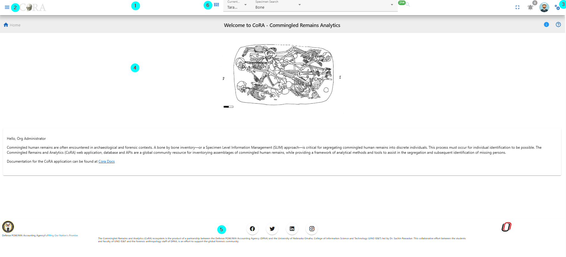
The navigation bar consists of the CoRA icon, toggle the left sidebar button, project switcher dropdown, advance search bar, the notifications icon, user profile avatar, and the right sidebar button.
- CoRA (1) - The CoRA icon take the user to the home page of the site.
- Toggle the Left Side bar (2) - The Toggle button opens and close the left sidebar.
- Project Dashboard (3) - This takes you to the project dashboard page.
- Project Switcher (4) - The Project switcher button allows the user to select the different projects the user is a part of.
- Advance Search bar (5) - The Advance search bar allows the user to search the Skeletal Elements,DNA, Dental, Missing Person, Isotope and Individual Number. The user can search the Skeletal Element by - Bone, Composite key, Accession, Provenance 1, Provenace 2, Designator, External ID, Individual Number. The DNA can be searched by the Bone, Composite Key, Accession, Sample Number, Mito seq Number, Haplogroup, External Id, Individual Number. The Isotope can be searched by Bone, Composite key, Accession, Provenance 1, Provenace 2, Designator, External ID, Individual Number. The Dental can be searched by Tooth and Dental Code. The Missing Person can be searched by Case manager, Case Status, Conflict, Genealogy status, First Name, Last Name. The Individual can be searched by Individual Number.
- Search Input (6) - Once the search type is selected the user can enter the value in the search input.
- Then click on the search icon, to go to the search page.
- Notification Icon (8) - The Notification icon show the notifications of the Export file, Import file, job completion and other user specific notification.
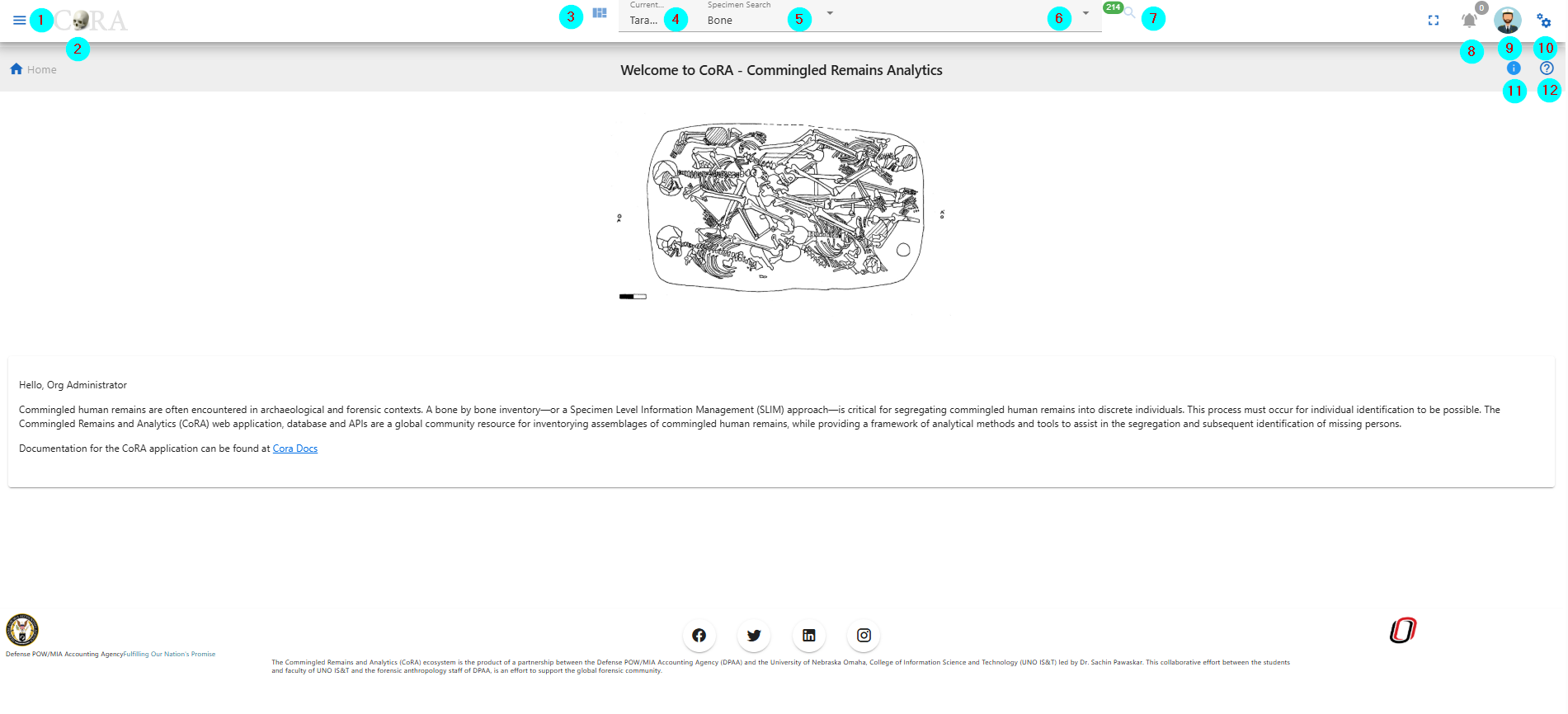
- User Avatar (9) - The user avatar shows the user drop down. The user drop down has User Image, User Name and Role (1), the github CoRA docs (2), CoRA Forum (3), CoRA Slack (4), change password link (5), the CoRA-Docs (6), the About (7), the My Profile button (8), Org Profile button (9) and the Logout button (10). The Org Profile button will only be available to the Org admin in which the Org Admin can change the settings of the project.
The header (1) shows the User Image, User Name, email and Role. Github CoRA docs (2) opens the github repo on which the user can check the documentation code. CoRA Forum (3) allows the user to leave comments and other related information about the cora eco system. CoRA Slack (4) allows users and developers to communicate and have private group discussion. The change password link (5) allows the user to change the current password. Online help (6) opens the online help documentation of the CoRA web application, it includes the user manual and other important docs. The About (7) displays the meta data of the application, the browser and the ability to clear the application cache. The My Profile button (8) open the user profile page in which the user can save the settings of their choice. The Org Progile button (9) shows information about the org. The Logout button (10) logs out the user out of CoRA Web Application. - Right Sidebar Toggle Button (10) - The Right sidebar buttons toggles between the open and closed state of right sidebar.
- Info tip for page the user is on.
- Help page for the page the user is on.
Search Capability
As a user you can search by the main categories listed below. Once an option and criteria are selected, the user can then click the search function (magnifyinging glass icon). The user will then be taken to the correct results page with detialed information, or the page will display 'No Data' if their search didn't bring back any information.
Search Categories:
- Specimen
- DNA
- Isotope
- Dental
- Missing Person
- Individuals
!!! Tip The search results will only show data for the project the user currently has selected. All search results are limited to the user permissions to view or access the data.
For more information on search Search User Guide
Left Side Drawer
Module Navigaion Menu
The left side bar includes the various modules of the CoRA web application that the user can select. The left side bar will have modules according to the role of the user. The following section shows the left side bar, each menu section is driven by role permissions.
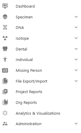
-
The Dashboard icon takes the user to the dashboard based on the user-role. If the user is Anthropologist then the Anthropologist dashboard will open and if the user iss Org-Admin the Org-Admin Dashboard will open. The dashboard page contains data visualization of the specimens data and dna module. The data visualization has pie charts, bar charts, stacked bar charts and other visualization The view details button on each visualization shows the data associated with that visualization.
-
The Specimen icon open the specimen elements module features like New Specimen Elements, New Bone Group, Skeletal Elements Reports. The New Skeletal Elements opens the page to add the new skeletal element. The New Bone Group opens the page that allows the user to add new skeletal element bone group. The Reports dashboard opens the reports dashboard page which allows the user to generate the reports based on the skeletal elements details.
-
The DNA icon opens the DNA features like Search the specimen element by DNA and Mitochondrial DNA - Advanced Report page.
- The Isotope icon opens up the Isotope features like view isotopes, isotope batches, create a new isotope batch and the isotope dashboard.
- The Dental icon opens the Dental features like create a new dental specimen, by new tooth, multiple via bone group and multiple via dental chart and view by missining person comparison report.
- The Individual icon opens up the Individual features like view by individual management report, and view the individual analytic dashbaord.
- The Missing Person icon opens up the Missing Person features like advance reporting, and Missing Person dashboard.
- The File Export/Import icon opens up the File Export/Import features like file export, file import, and file manager.
- The Project Reports icon opens up the Project Reports for the project you are currently viewing.
- The Org Reports icon opens up the Org Reports for the org you are currently viewing.
- The Analytics & Visualizations icon opens up the Analytics & Visualizations dashboard with visualizations and analytics.
- The Administration icon opens up the Administration features for the role of the user.
Right Side Drawer
The Right side bar includes the 4 different sections and each of the section includes the user specific settings. The following are the sections in the right side bar.
- Layout Options
- Help
- Activity Feed
- General Settings
![]()
Layout Options
Layout Options Section includes the Scheme(1), Drawer(2) and Footer (3).
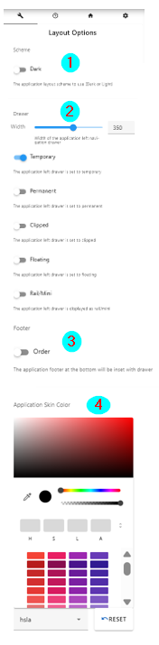
The Scheme option allows the user to select between the dark theme or light theme. The default theme is light theme. The dark theme color changes the top navigation bar color. The light theme changes the top navigation color and the left side bar theme color to light.
The Layout Options (2) allows the user to make changes in the layout of the app. The following are the description of the options in layout-
Toggle Side Bar (1)- The Toggle Sidebar checkbox open and close the left sidebar. If checked the left side bar will open and if unchecked the left sidebar will be closed. Left Sidebar Expand on Hover (2)- This option allows the user to allow the user to show the left sidebar menu on mouseover. Toggle Right Sidebar Slide (3)- This options allows the app container to move left. It allows the user to work simultaneously on right side bar tabs and the main app content. Toggle Right Sidebar Skin (4)- This options allows the user to toggle between the light and dark background theme on right side bar.
Help
Help section (2) - The Help section allows the user to access the CoRA-Docs inside the right side bar.

The documentation of the CoRA application along with the user manual can be found in this tab. The Menu button can be clicked to select the different sections of the documentation.
Activity Feed
The Activity feed section shows the 10 recent Skeletal Elements and DNA created and updated by the user.

The key can be of the skeletal element can be clicked which takes the user to the selected skeletal element so, that the user can easily access the recently added skeletal elements and update it if needed. This activity feed can also be found in user profile under the activity feed tab.
General
The General section allows the user to customize the user settings.

The Lines per page (1) allows the user to select the number of rows to be display for views with table. The user can set this value from the user profile as well.
The Skeletal Element setting (2) allows the user to set the Accession Number, Provenance 1 and Provenance 2. This value will auto fill the value whenever new skeletal element is created.
The DNA Profile settings (3) in the Gerenal tab allows the user to update the default laboratory and Default DNA Method. Once the user enter the value it will auto-populate the DNA association screen for Skeletal Elements.
Application Container
The Application container is the main area which includes all the CoRA-Modules.
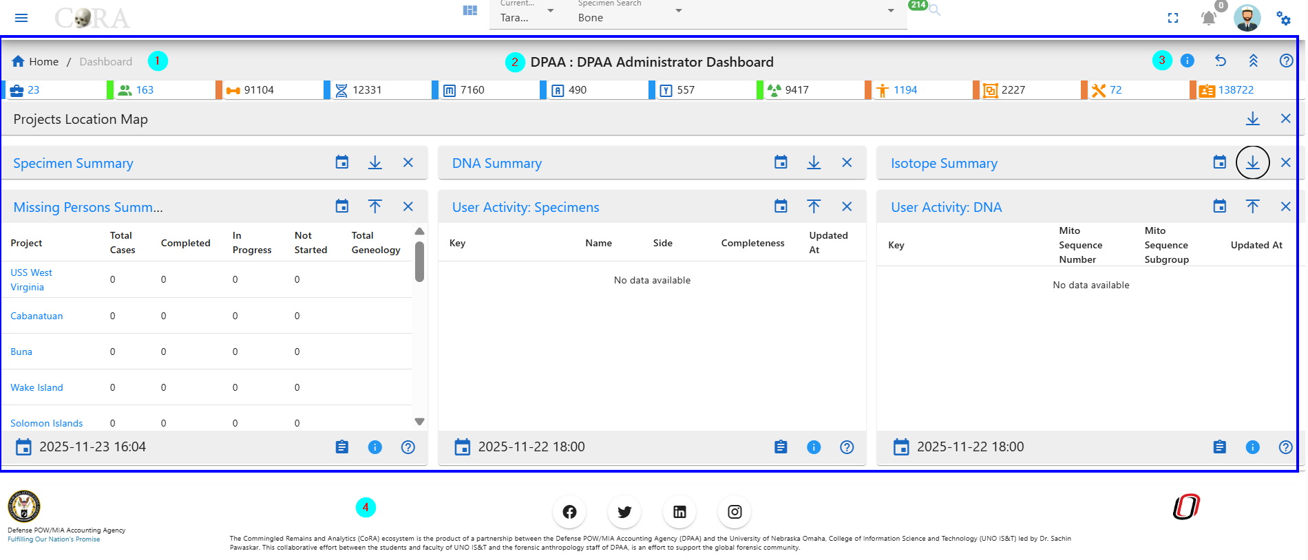
Breadcrumbs
The Application container has Breadcrumbs (1) on the top left which shows on which page the user is currently working on. It helps the user to go back to the last page.
Page title
The Title of the page (2) the user is working on.
Action button group
The Action button group (3). This button may or may not be present based on the page the user is working on. If the page has no action this button will not be present.
Footer
The footer (4) consists of the logos and product information
Org Users Projects
The CoRA application is structured around the concept of organization, users and projects. What does this mean for you? CoRA was designed to be used by both organizations and single users. Organizations can be government organizations, non-profits, universities or any entity that deals with the identification of missing persons, or segregation of human remains. Single users could be any single individual who wants to use CoRA for their own project, a use case might be for university students of forensic anthropology.
erDiagram
  ORG ||--o{ PROJECT : has
  ORG {
    string name
    string description
    string acronym
  }
  PROJECT ||--|{ SPECIMEN : contains
  PROJECT {
    string name
    string description
  }
  SPECIMEN {
    id bone
    string side
  }
  ORG }|--|{ USER : belongsTo
  USER {
    string name
    id role
  }
  USER }|..|{ PROJECT : assignedTo
Organizations
Organizations or simply "Orgs" in CoRA is a top level container. Orgs will usually have Users and Projects and Org Administrators can create these users and projects within that org and most importantly assign users to projects. The org administrator is also responsible to managing and updating the org profile which are attributes and settings that apply to all projects and users as well can control settings within CoRA.
Users
Users in CoRA belong to a org and user accounts are created are typically assigned to projects by the org administrator. Anyone who uses CoRA must have a user account and must be assigned a role (such as org administrator, anthropologist, dna analyst, isotope analyst, dentist, historian, etc). Each role provide a specific level of authorization to features within CoRA. The users are responsible for managing and updating their user profile which are attributes that can control user settings within CoRA.
Projects
Projects in CoRA is a container that holds specimens. In CoRA specimens must belong to a project and projects themselves belong to an org. Project attributes and settings can be controlled and managed by the project manager who is typically an anthropologist who is also assigned to that project.
Org Administrator
Every Org must have an Org Administrator (Org Admin for short) who is one of the Users with a privileged role. The Org Admin has the ability to create and manage the Users, Projects, Accession, Instruments, Haplogroups etc. Users with the Org Administrator role will be presented with the Administration menu to perform these functions. Lets look at some of these functions
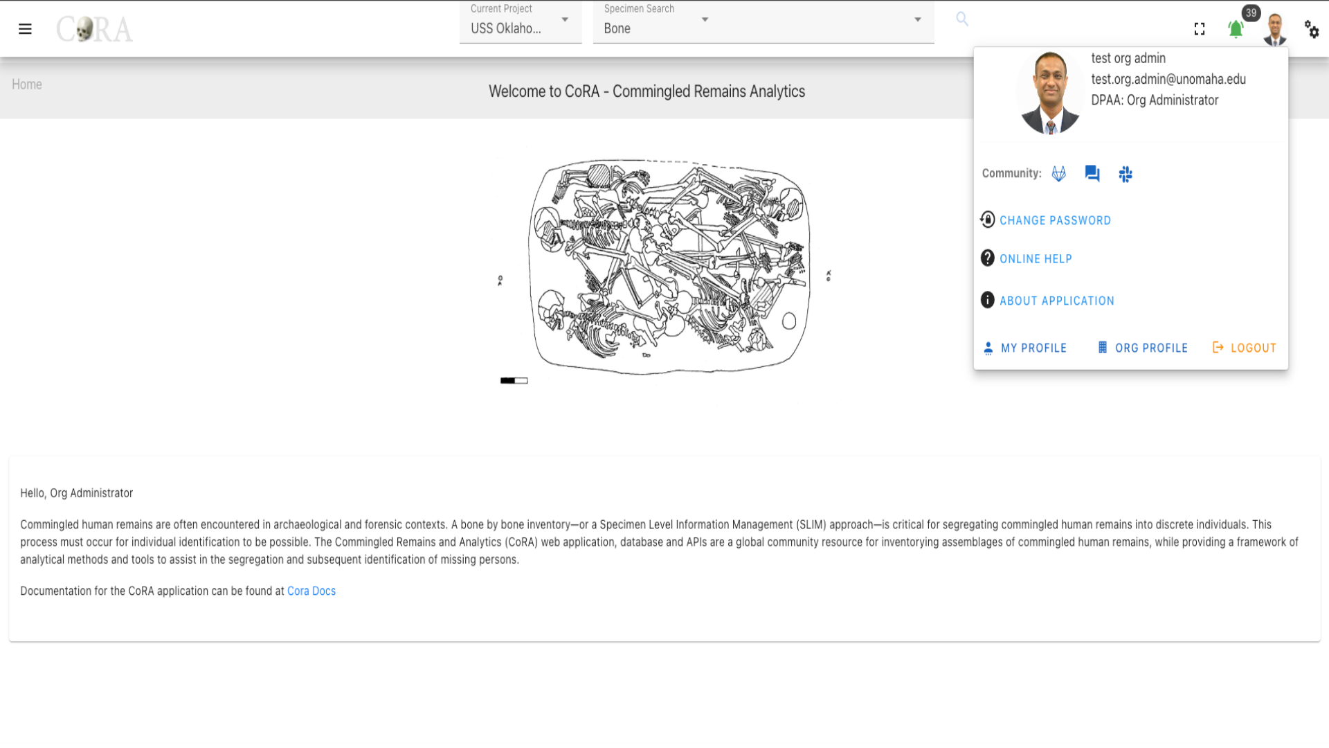
Navigation to Administration
An Org Admin can click on the hamburger and go to 'Administration' to find all the Administration pages.
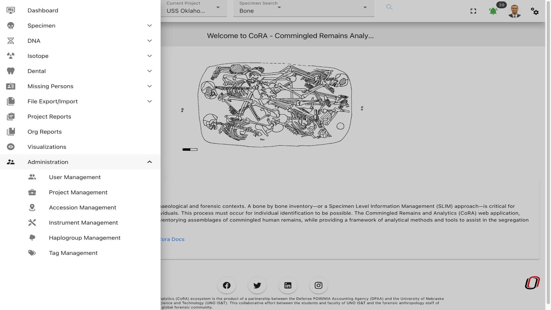
User Management
The Org Administrator has the ability to browse users list, create and manage the users along with the ability to assign users to projects. The user management screen provides a data table of all the users with information such as Name, Role, Email, Cell Phone, Active Status, Country, Language, Time Zone, IP Address, Last Activity, etc. The users list will be initially sorted on the user name and email. The data table also has an "Actions" column with buttons to reset the password, reset in-activity lock and edit the user record.
Tip
- You can edit the user by clicking the user name link.
- The column visibility will allow you to add more columns/details to the data table list.
- The Search box can be used to search any details in the data table list.
Create User
On the user management screen, click the Create button/icon to create a new user. Navigation to the user Management screen is shown below.
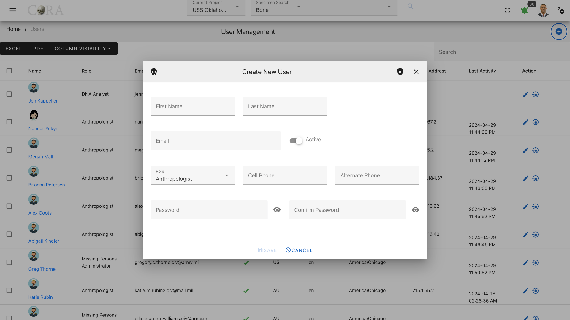
The Create button opens a dialog box to prompt to create a new user. Enter the information for the new user record, including the the "Role" field. Various user roles can be selected such as Org Admin, Anthropologist, Manager, DNA Analyst, Historian, Isotope Analyst. Intern, etc. Once all information is entered, click "Save", and a success message “User successfully added” will appear at the top.
The screen fields are shown below. Fields in bold are required.
| Attributes | Data Type | Size | Validation Rule | Required/Optional |
|---|---|---|---|---|
| First Name | String | 32 chars | contains letters | Required |
| Last Name | String | 32 chars | contains letters and dash | Required |
| String | 255 chars | max 255, unique | Required | |
| Role | Id | valid option via dropdown | Required (Default Anthropologist) | |
| Active Status | Boolean | true/false toggle | Required (Default Active) | |
| Cell phone | String | 32 chars | contains numbers and dash | Optional |
| Alternate phone | String | 32 chars | contains numbers and dash | Optional |
| Password | String | 64 chars | min 10, at least 1 letter, 1 cap, 1 number, 1 special | Required |
| Confirm Password | String | 64 chars | min 10, at least 1 letter, 1 cap, 1 number, 1 special | Required |
Note
Users will be able to change their password once they have logged in. Ensure to check the Active box so that the user account is active and the user can login.
Note
After the user has been created the Org Administrator must assign that user to at least one project.
Edit User
To edit an existing users information, simply click on the Name and the edit dialog box will open for editing the existing user information. The following fields are available for update, click "Save" when finished editing, or "Close" to cancel the changes.
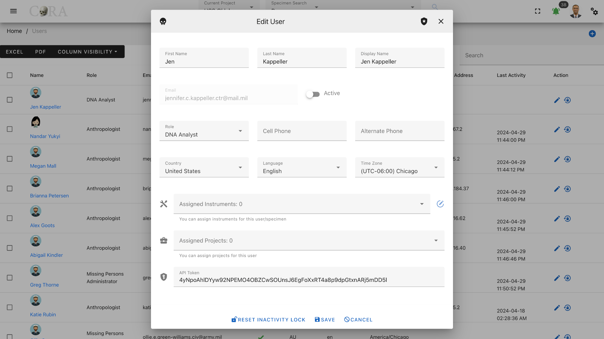
The screen fields are shown below. Fields in bold are required.
| Attributes | Data Type | Size | Validation Rule | Required/Optional |
|---|---|---|---|---|
| First Name | String | 32 chars | contains letters | Required |
| Last Name | String | 32 chars | contains letters and dash | Required |
| Last Name | String | 32 chars | contains letters and dash | Optional |
| String | 255 chars | max 255, unique | Required | |
| Active Status | Boolean | true/false toggle | Required (Default Active) | |
| Role | Id | valid option via dropdown | Required (Default Anthropologist) | |
| Cell phone | String | 32 chars | contains numbers and dash | Optional |
| Alternate phone | String | 32 chars | contains numbers and dash | Optional |
| Country | String | valid option via dropdown | Required (Default United Stated) | |
| Language | String | valid option via dropdown | Required (Default English) | |
| Timezone | String | valid option via dropdown | Required (Default UTC-06:00 Chicago) | |
| Instruments | Id | valid options via dropdown | Optional | |
| Projects | Id | valid options via dropdown | Required (at least one) | |
| API Token | String | 255 chars | valid token string | Optional/Required for API |
Batch Edit Users
The user management screen allows for batch editing of multiple user records. This can be useful to administrators for passwords resets, change user active status flag, etc. To batch edit, select multiple users by clicking on the boxes to the left of their names, this will show the "Actions" menu in the top-left menu, select the Actions > Batch Edit menu.
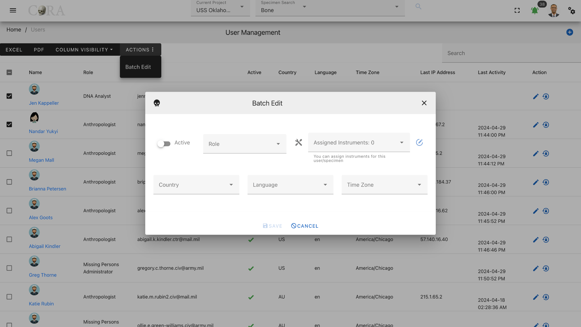
The screen fields for batch edit are shown below.
| Attributes | Data Type | Size | Validation Rule |
|---|---|---|---|
| Active Status | String | 32 chars | contains letters |
| Assigned Instrument | String | 32 chars | contains letters and dash |
| Country | String | valid option via dropdown | |
| Language | String | valid option via dropdown | |
| Timezone | String | valid option via dropdown |
User Access
If a user has too many incorrect login attempts, the user will be unable to log in for the lockout period. Currently, the number of incorrect login attempts is set to 3, and the lockout period is 10 minutes.
If a user is inactive for too many days (configured by organization), their account will be suspended, and a lock icon will appear next to their last activity date in the User Management screen. The default value for inactive days resulting in suspension is 60 days.
To reactivate their account, click on the Reset Inactivity Lock icon, an open the padlock, on the far right side of the user row.
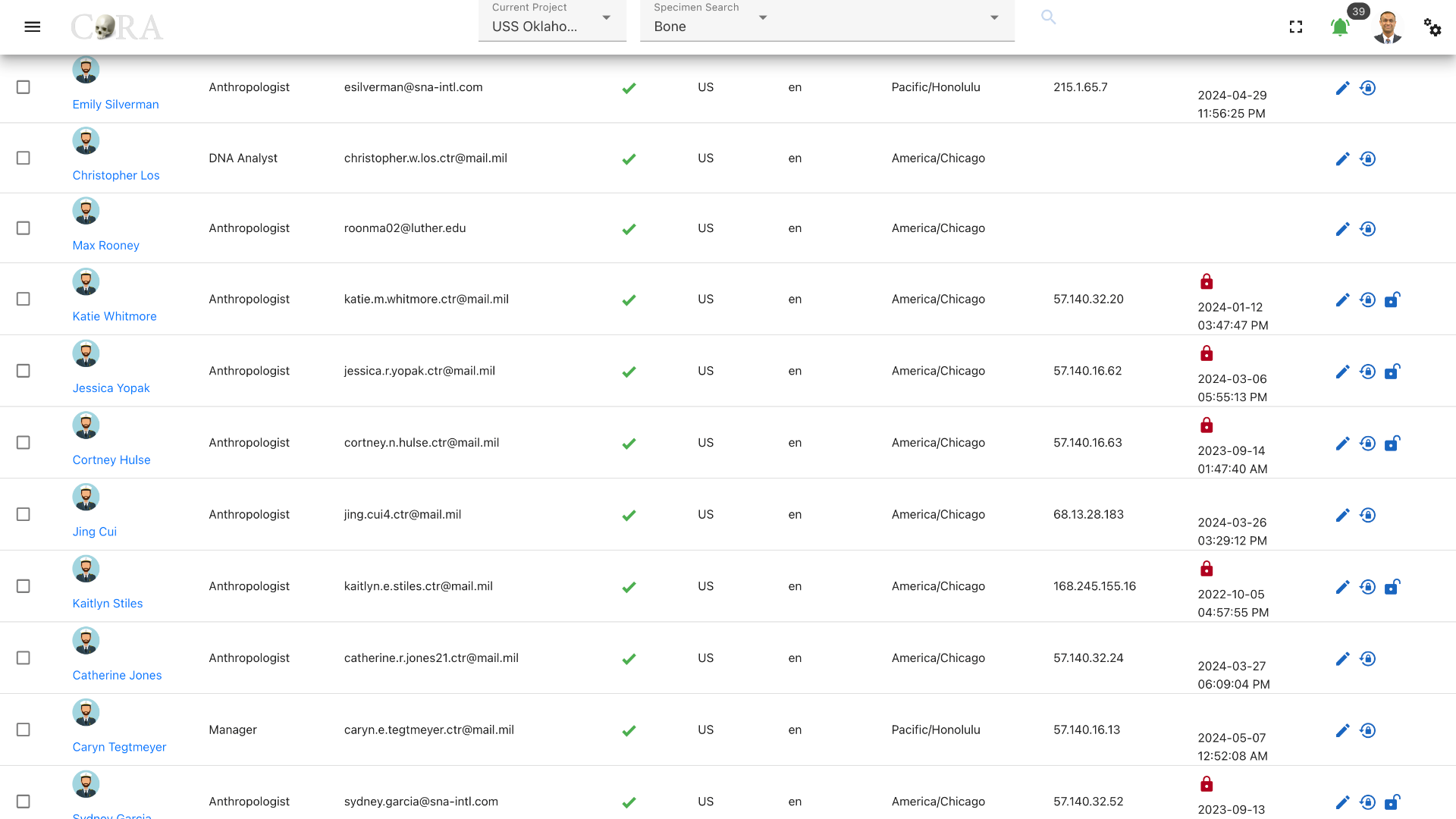
To reactivate multiple accounts, select multiple users by clicking on the boxes to the left of their names. Then, select Actions in the top-left menu, then click on Batch Edit. In the popup, click on Reset Inactivity Lock.
To reset an account password, click on the Password Reset icon to open the Reset Password dropbox. Enter the new password and confirm the newly entered password to reset the password
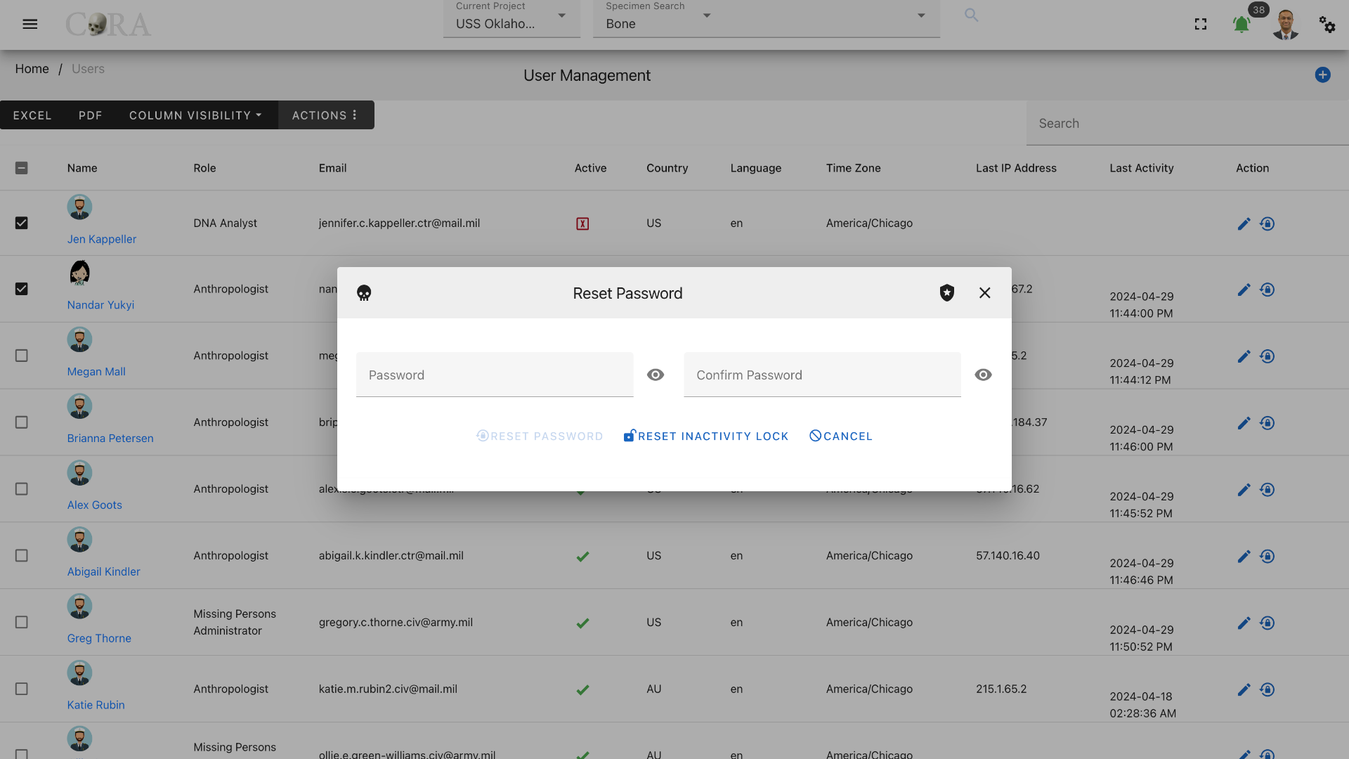
The screen fields are shown below. Fields in bold are required.
| Attributes | Data Type | Size | Validation Rule | Required/Optional |
|---|---|---|---|---|
| Password | String | 32 chars | contains letters | Required |
| Confrim Password | String | 32 chars | contains letters and dash | Required |
Project Management
The Org Administrator has the ability to browse project list, create and manage the projects along with the ability to assign users to projects. The project management screen provides a data table of all the projects with information such as Name, Description, Manager, Start Date, Status and whether it is Public or not. The projects list will be initially sorted on the project name. The data table also has an "Actions" column with buttons to edit the project.
Tip
- You can edit the project by clicking the project name link.
- The column visibility will allow you to add more columns/details to the data table list.
- The Search box can be used to search any details in the data table list.
Create Project
On the project management screen, click the Create button/icon to create a new project. Navigation to the project management screen is shown below.
The Create button opens a dialog box to prompt to create a new project. Enter the information for the new project record, including the the "Manager" field. Once all information is entered, click "Save", and a success message “Project successfully added” will appear at the top.
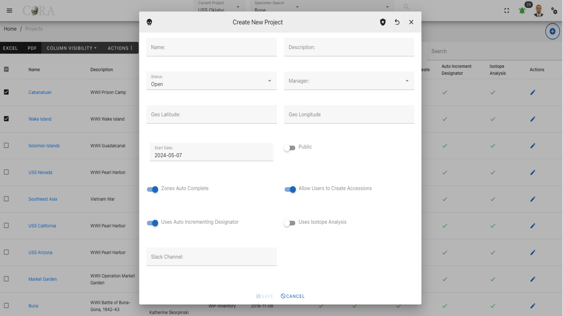
The screen fields are shown below. Fields in bold are required.
| Attributes | Data Type | Size | Validation Rule | Required/Optional |
|---|---|---|---|---|
| Name | String | 255 chars | contains letters and numbers, min:3 and max:255 | Required |
| Description | String | 255 chars | contains letters and numbers | Required |
| Status | Id | valid option via dropdown | Required (Default Open) | |
| Manager | Id | valid option via dropdown | Required | |
| Geo latitude | Decimal | valid lat/long up to 7 decimal precision | Required | |
| Geo Longitude | Decimal | valid lat/long up to 7 decimal precision | Required | |
| Start Date | Date | valid date | Required | |
| Public | Boolean | true/false toggle | Required (Default false) | |
| Zones Auto Complete | Boolean | true/false toggle | Required (Default true) | |
| Allow Users to Create Accessions | Boolean | true/false toggle | Required (Default true) | |
| Uses Auto Incrementing Designator | Boolean | true/false toggle | Required (Default true) | |
| Isotope Analysis | Boolean | true/false toggle | Required (Default false) | |
| Slack Channel | String | 255 chars | valid url | Optional |
Warning
If the project is flagged as Public, your project will be visible to all. This option is rarely used and is only available in case you want to share your project with others not part of your organization.
Edit Project
To edit an existing projects information, simply click on the Name and the edit dialog box will open for editing the existing project information. The following fields are available for update, click "Save" when finished editing, or "Close" to cancel the changes.
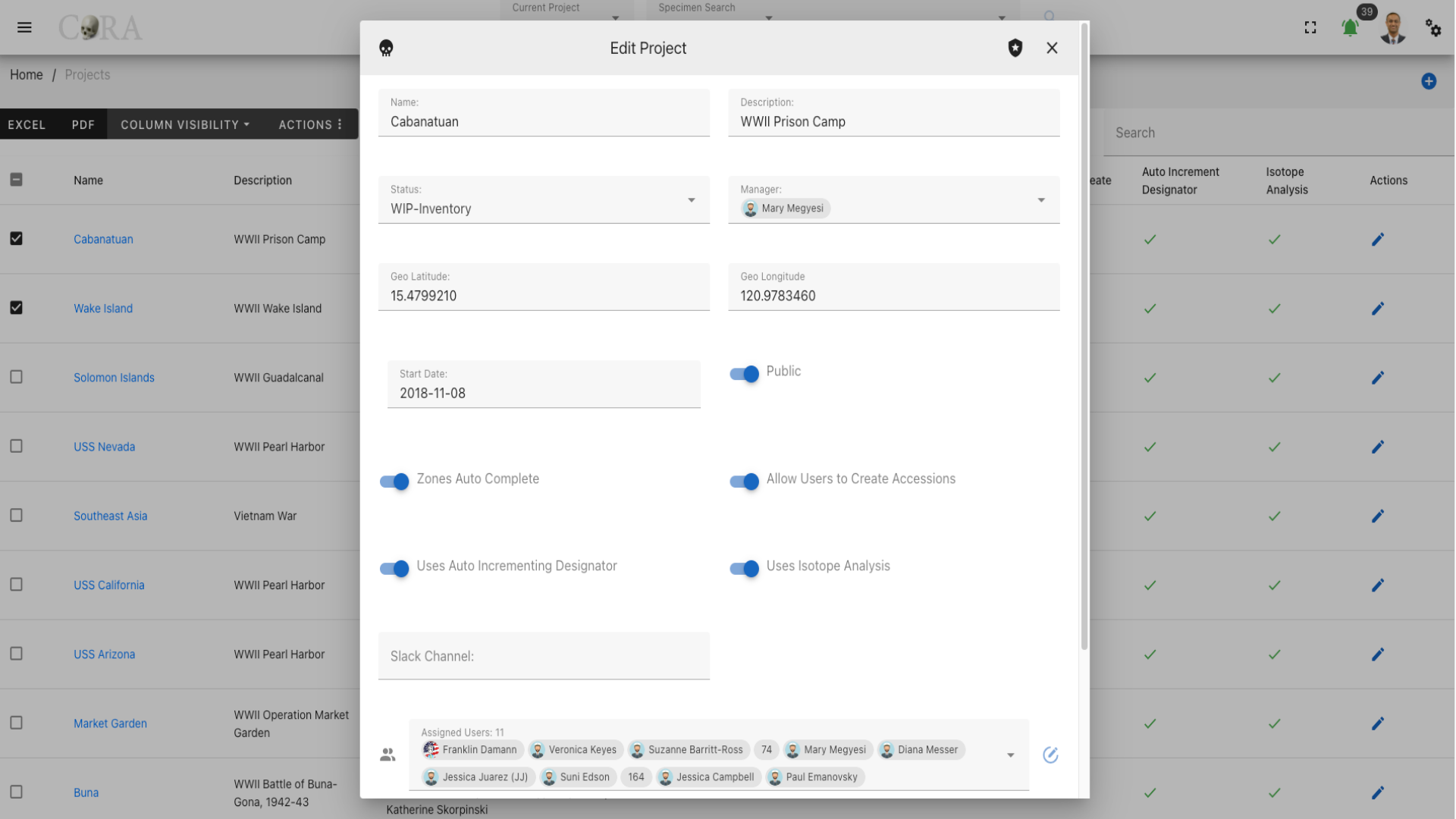
The screen fields are shown below. Fields in bold are required.
| Attributes | Data Type | Size | Validation Rule | Required/Optional |
|---|---|---|---|---|
| Name | String | 255 chars | contains letters and numbers, min:3 and max:255 | Required |
| Description | String | 255 chars | contains letters and numbers | Required |
| Status | Id | valid option via dropdown | Required (Default Open) | |
| Manager | Id | valid option via dropdown | Required | |
| Geo latitude | Decimal | valid lat/long up to 7 decimal precision | Required | |
| Geo Longitude | Decimal | valid lat/long up to 7 decimal precision | Required | |
| Start Date | Date | valid date | Required | |
| Public | Boolean | true/false toggle | Required (Default false) | |
| Slack Channel | String | 255 chars | valid url | Optional |
| Zones Auto Complete | Boolean | true/false toggle | Required (Default true) | |
| Allow Users to Create Accessions | Boolean | true/false toggle | Required (Default true) | |
| Uses Auto Incrementing Designator | Boolean | true/false toggle | Required (Default true) | |
| Isotope Analysis | Boolean | true/false toggle | Required (Default false) | |
| Latest MCC Date* | Date | valid date | Optional | |
| Assigned Users | Id | valid options via dropdown | Required (at least one) | |
| Assigned Instruments | Id | valid options via dropdown | Optional |
Batch Edit Project
The Project Management screen allows for batch editing of multiple project records. This can be useful to change project status,to make a public, etc. To batch edit, select multiple projects by clicking on the boxes to the left of their names, this will show the "Actions" menu in the top-left menu, select the Actions > Batch Edit menu. this will open a batch edit dropbox.
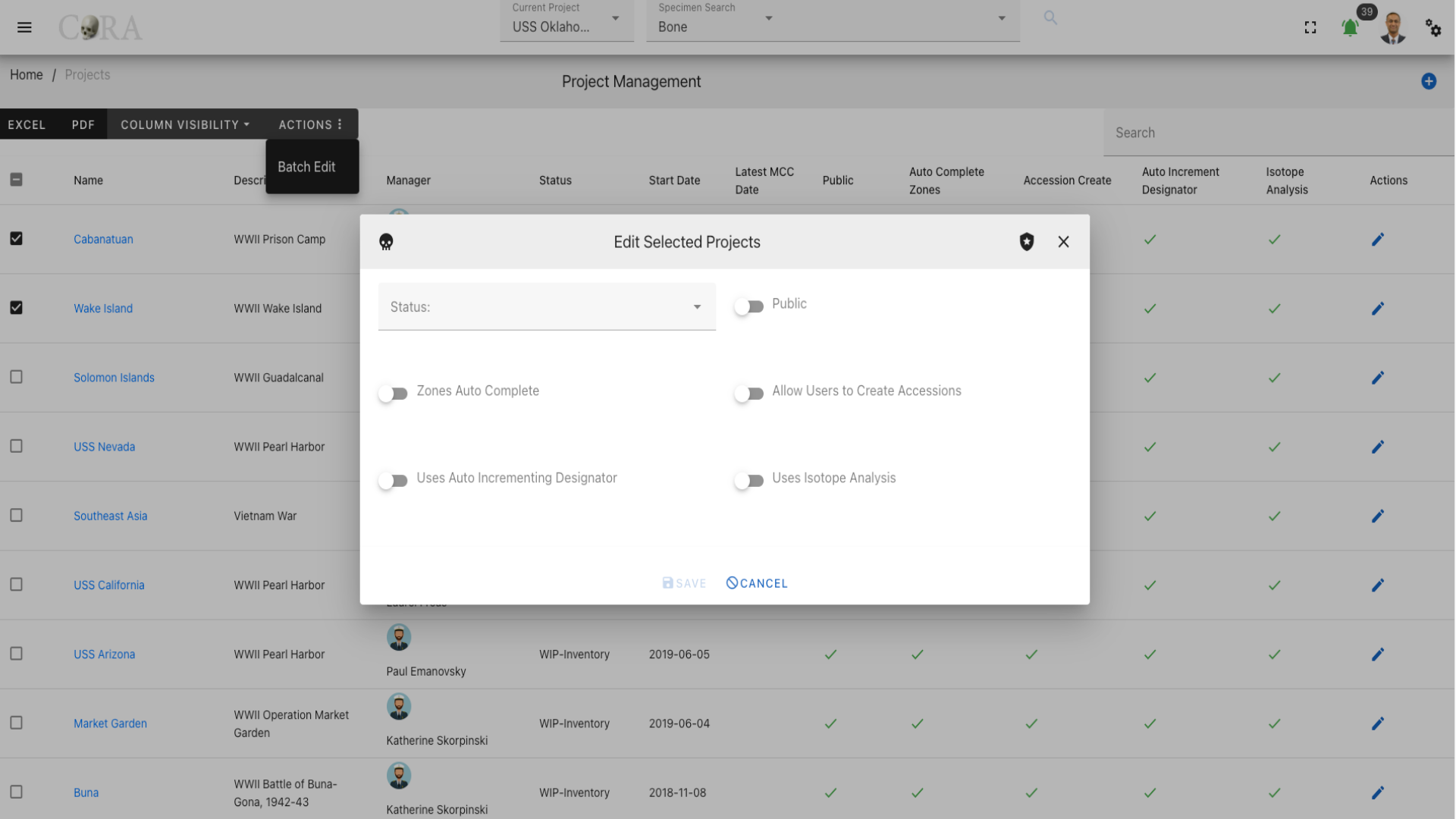
The screen fields for batch edit are shown below.
| Attributes | Data Type | Size | Validation Rule |
|---|---|---|---|
| Status | String | 32 chars | contains letters |
| Public | Boolean | true/false toggle | |
| Zones Auto Complete | Boolean | true/false toggle | |
| Allow Users to Create Accessions | Boolean | true/false toggle | |
| Uses Auto Incrementing Designator | Boolean | true/false toggle | |
| Isotope Analysis | Boolean | true/false toggle |
Accession Management
The Org Administrator has the ability to browse accession list, create and manage the accessions along with the ability to assign accessions to projects. The accession management screen provides a data table of all the accessions in the current project with information such as Project Name, Key, Number, Provenance 1, and Provenance 2. The accessions list will be initially sorted on the project name. The data table also has an "Actions" column with buttons to edit the accession.
Tip
- You can edit the accession by clicking the accession key link.
- The column visibility will allow you to add more columns/details to the data table list.
- The Search box can be used to search any details in the data table list.
Create Accession
On the accession management screen, click the Create button/icon to create a new accession. Navigation to the accession management screen is shown below.
The Create button opens a dialog box to prompt to create a new accession. Enter the information for the new accession record, the "Project" field is defaulted to current project. Once all information is entered, click "Save", and a success message Accession successfully added” will appear at the top.
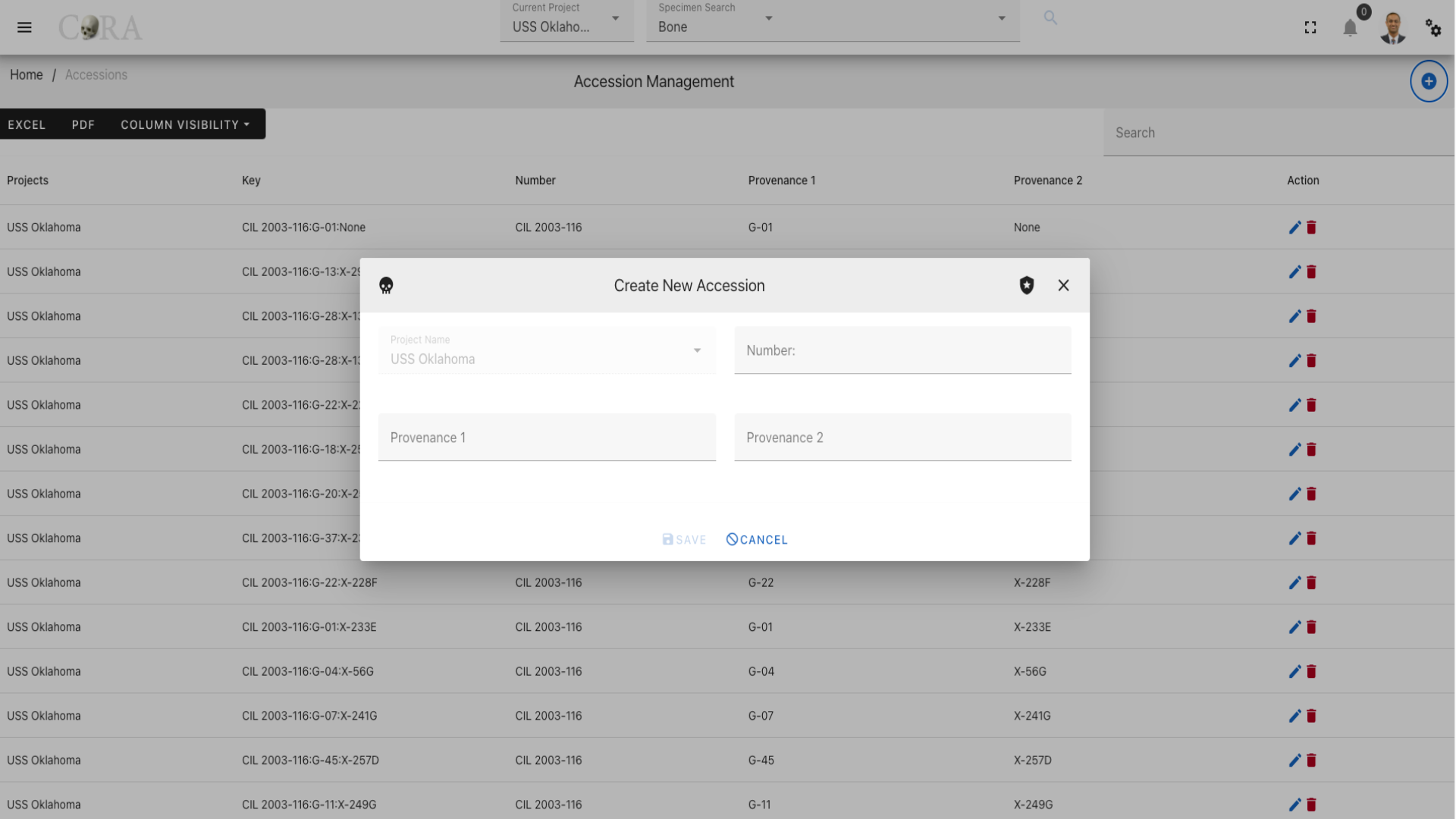
The screen fields are shown below. Fields in bold are required.
| Attributes | Data Type | Size | Validation Rule | Required/Optional |
|---|---|---|---|---|
| Project | Id | valid option via dropdown | Required (Default current project) | |
| Number | String | 32 chars | contains letters and numbers | Required |
| Provenance1 | String | 32 chars | contains letters and numbers | Optional |
| Provenance2 | String | 32 chars | contains letters and numbers | Optional |
Edit Accession
To edit an existing accession information, simply click on the Key and the edit dialog box will open for editing the existing accession information. The following fields are available for update, click "Save" when finished editing, or "Close" to cancel the changes.
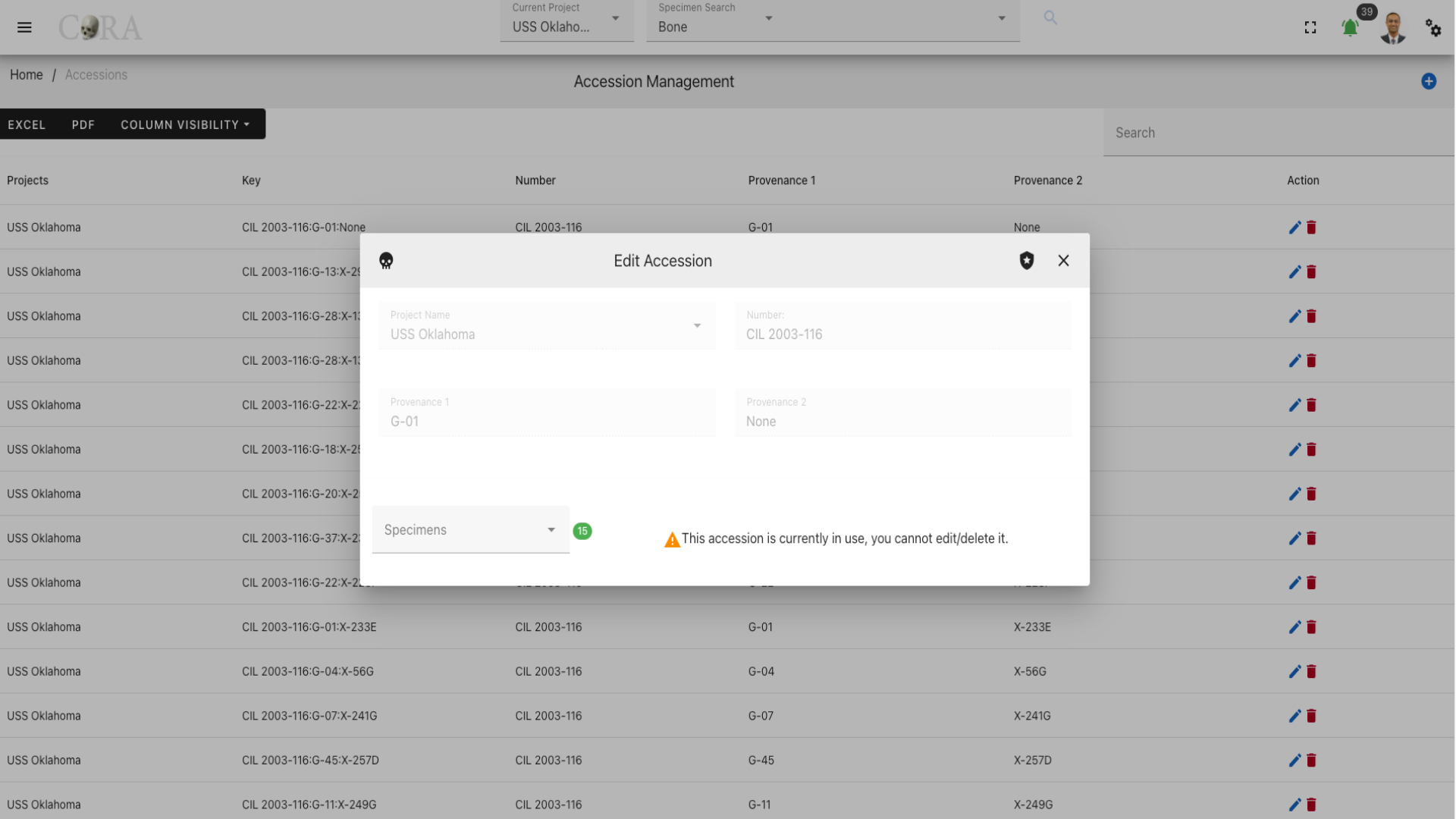
The screen fields are shown below. Fields in bold are required.
| Attributes | Data Type | Size | Validation Rule | Required/Optional |
|---|---|---|---|---|
| Project | Id | valid option via dropdown | Required (Default current project) | |
| Number | String | 32 chars | contains letters and numbers | Required |
| Provenance1 | String | 32 chars | contains letters and numbers | Optional |
| Provenance2 | String | 32 chars | contains letters and numbers | Optional |
| Specimens | String | 32 chars | contains letters and numbers |
Note
If there are specimens under an accession, then the specimens and their count are displayed along with a message "This accession is currently in use, you cannot edit/delete it."
Tip
If you want to edit or delete an accession please make sure that all specimens under that accession have first been reassigned and another accession and the current count is 0 before attempting to edit or delete an accession.
Instrument Management
The Org Administrator has the ability to browse instrument list, create and manage the instruments along with the ability to assign instruments to users. The instrument management screen provides a data table of all the instruments in the current organization with information such as Code, Module, Active Status, Category, Reference and Assigned Users. The instruments list will be initially sorted on the code and module. The data table also has an "Actions" column with buttons to edit the instrument.
Tip
- You can edit the instrument by clicking the code link.
- The column visibility will allow you to add more columns/details to the data table list.
- The Search box can be used to search any details in the data table list.
Create Instrument
On the instrument management screen, click the Create button/icon to create a new instrument. Navigation to the instrument management screen is shown below.
The Create button opens a dialog box to prompt to create a new instrument. Enter the information for the new instrument record, the "Active Status" field is defaulted to true. Once all information is entered, click "Save", and a success message Instrument successfully added” will appear at the top.
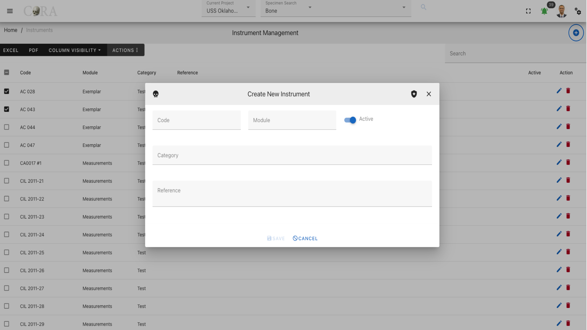
The screen fields are shown below. Fields in bold are required.
| Attributes | Data Type | Size | Validation Rule | Required/Optional |
|---|---|---|---|---|
| Code | String | 16 chars | contains letters and numbers | Required |
| Module | String | 32 chars | contains letters and numbers | Required |
| Active Status | Boolean | true/false toggle | Required (Default true) | |
| Category | String | 255 chars | contains letters and numbers | Required |
| Reference | String | 255 chars | contains alphanumeric values | Optional |
Edit Instrument
To edit an existing instrument information, simply click on the Code and the edit dialog box will open for editing the existing instrument information. The following fields are available for update, click "Save" when finished editing, or "Close" to cancel the changes.
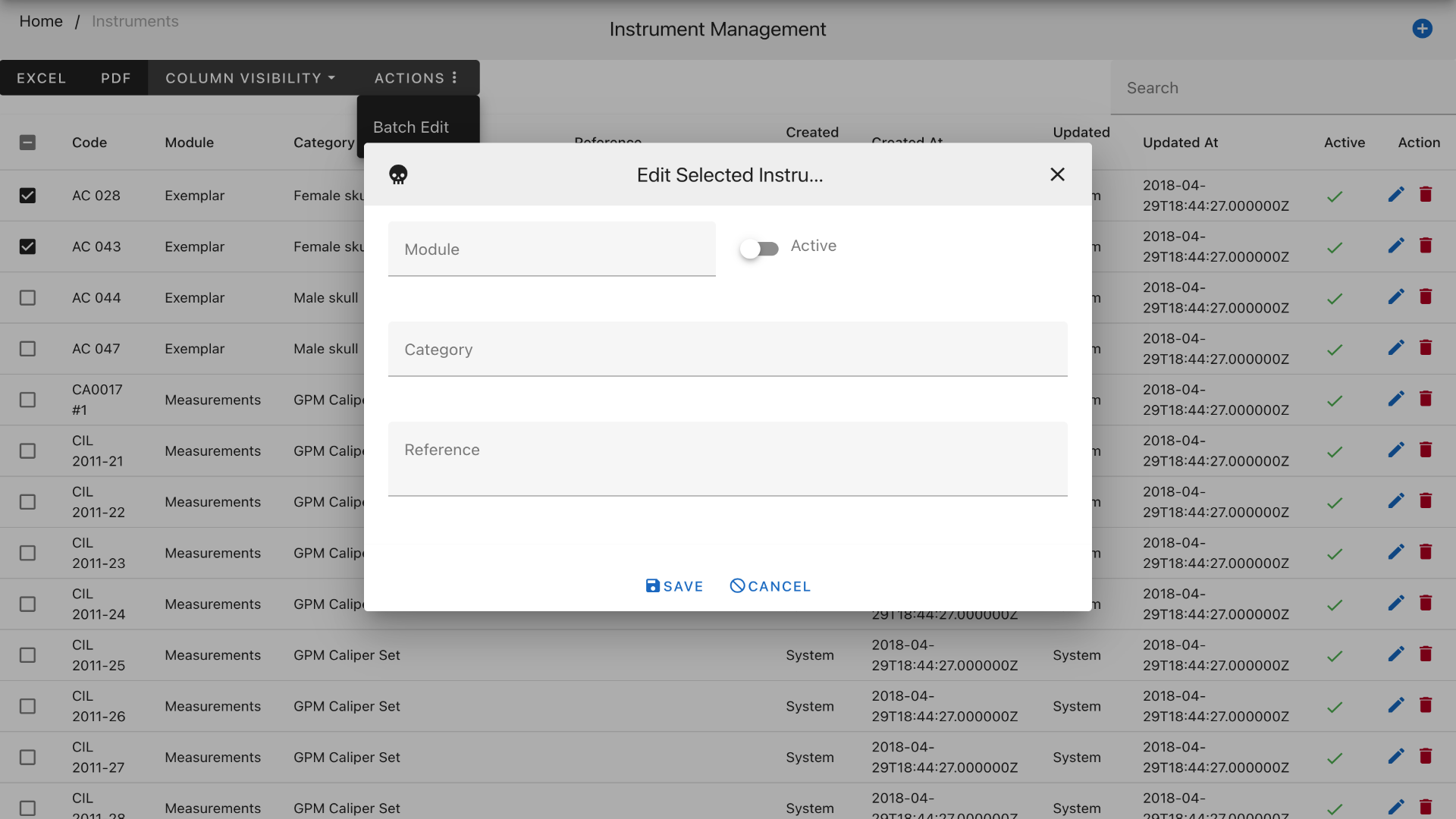
The screen fields are shown below. Fields in bold are required.
| Attributes | Data Type | Size | Validation Rule | Required/Optional |
|---|---|---|---|---|
| Code | String | 16 chars | contains letters and numbers | Required |
| Module | String | 32 chars | contains letters and numbers | Required |
| Active Status | Boolean | true/false toggle | Required (Default true) | |
| Category | String | 255 chars | contains letters and numbers | Required |
| Reference | String | 255 chars | contains alphanumeric values | Optional |
| Assigned Users | Id | valid options via dropdown | Optional |
Batch Edit Instrument
The Instrument Management screen allows for batch editing of multiple instruments. To batch edit, select multiple instruments by clicking on the checkboxes to the left of their names, this will show the "Actions" menu in the top-left menu, select the Actions > Batch Edit menu. this will open a batch edit dropbox.
![Click on Action]site-navigation/media/instrument-management-batch.png)
The screen fields for batch edit are shown below.
| Attributes | Data Type | Size | Validation Rule |
|---|---|---|---|
| Module | String | 32 chars | contains letters and numbers |
| Active Status | Boolean | true/false toggle | |
| Category | String | 255 chars | contains letters and numbers |
| Reference | String | 255 chars | contains alphanumeric values |
Haplogroup Management
The Org Administrator has the ability to browse haplogroup list, create and manage the haplogroups. The haplogroup management screen provides a data table of all the haplogroups in the current organization with information such as Type, Letter, Subgroup, and Ancestry. The haplogroups list will be initially sorted on the type and letter. The data table also has an "Actions" column with buttons to edit the haplogroup.
Tip
- You can edit the haplogroup by clicking the letter link.
- The column visibility will allow you to add more columns/details to the data table list.
- The Search box can be used to search any details in the data table list.
Create Haplogroup
On the haplogroup management screen, click the Create button/icon to create a new haplogroup. Navigation to the haplogroup management screen is shown below.
The Create button opens a dialog box to prompt to create a new haplogroup. Enter the information for the new haplogroup record. Once all information is entered, click "Save", and a success message Haplogroup successfully added” will appear at the top.
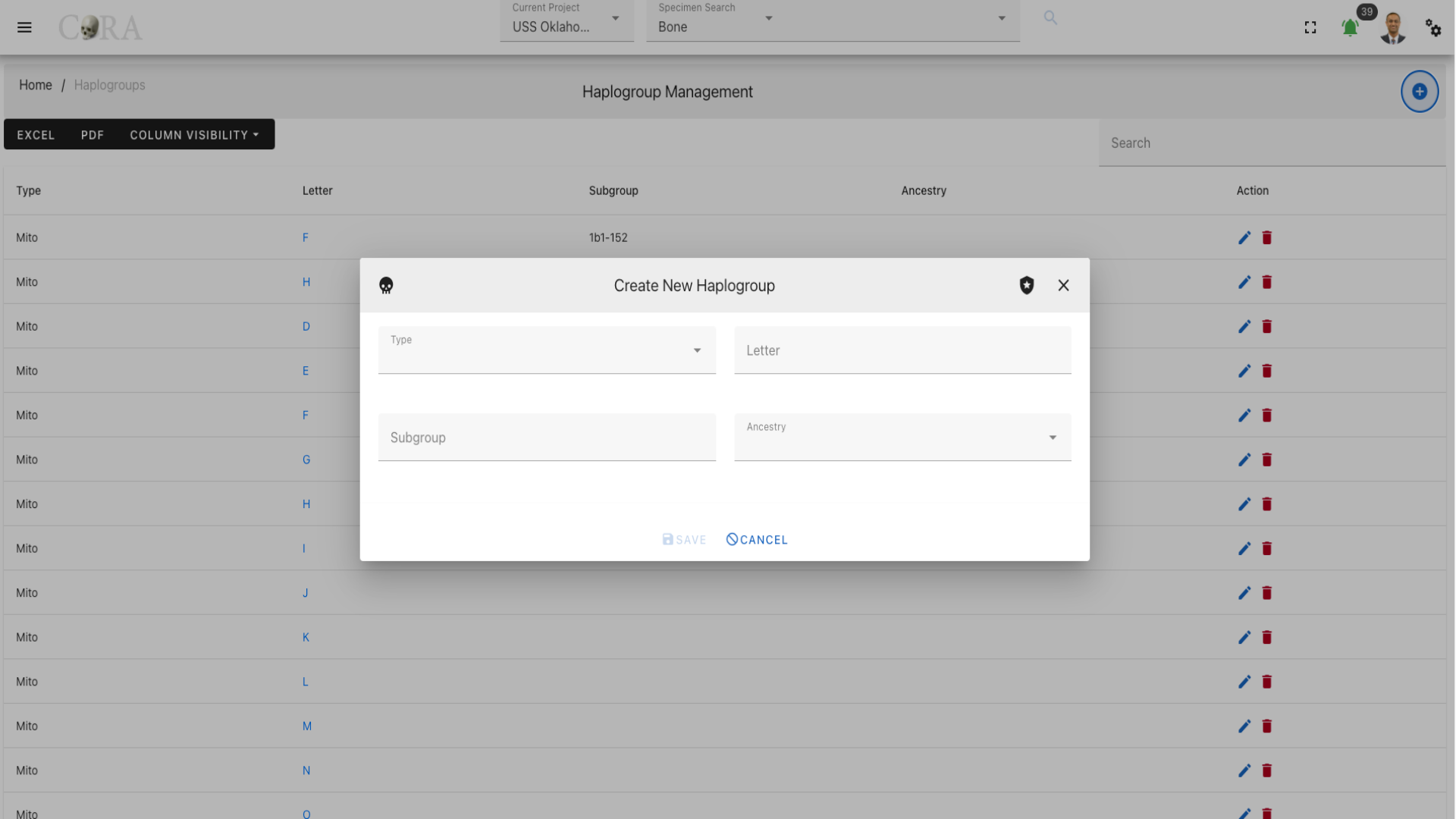
The screen fields are shown below. Fields in bold are required.
| Attributes | Data Type | Size | Validation Rule | Required/Optional |
|---|---|---|---|---|
| Type | String | 32 chars | valid options via dropdown (Mito, YStr) | Required |
| Letter | String | 1 char | contains letter, one char from A-Z | Required |
| Subgroup | String | 32 chars | contains alphanumeric values | Optional |
| Ancestry | String | 32 chars | valid options via dropdown | Optional |
Edit Haplogroup
To edit an existing haplogroup information, simply click on the Letter and the edit dialog box will open for editing the existing haplogroup information. The following fields are available for update, click "Save" when finished editing, or "Close" to cancel the changes.

The screen fields are shown below. Fields in bold are required.
| Attributes | Data Type | Size | Validation Rule | Required/Optional |
|---|---|---|---|---|
| Type | String | 32 chars | valid options via dropdown (Mito, YStr) | Required |
| Letter | String | 1 char | contains letter, one char from A-Z | Required |
| Subgroup | String | 32 chars | contains alphanumeric values | Optional |
| Ancestry | String | 32 chars | valid options via dropdown | Optional |
Tag Management
The Org Administrator has the ability to browse tags list, create and manage the tags along with the ability to assign tags to projects. The tags management screen provides a data table of all the tags in the current organization with information such as Name, Description, Category, Type, Color and Icon. The tags list will be initially sorted on the name. The data table also has an "Actions" column with buttons to edit the tag.
Tip
- You can edit the tag by clicking the name link.
- The column visibility will allow you to add more columns/details to the data table list.
- The Search box can be used to search any details in the data table list.
Create Tag
On the tag management screen, click the Create button/icon to create a new tag. Navigation to the tag management screen is shown below.
The Create button opens a dialog box to prompt to create a new tag. Enter the information for the new tag record. Once all information is entered, click "Save", and a success message Tag successfully added” will appear at the top.
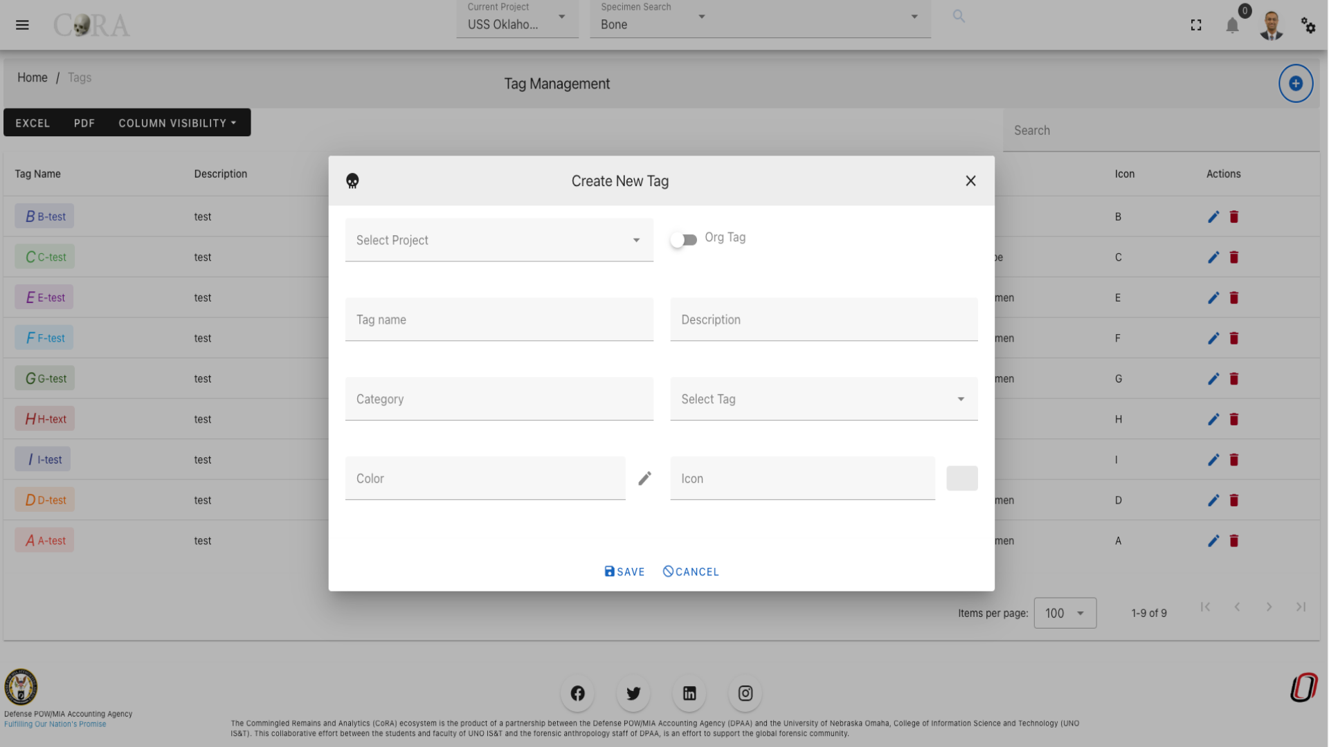
The screen fields are shown below. Fields in bold are required.
| Attributes | Data Type | Size | Validation Rule | Required/Optional |
|---|---|---|---|---|
| Project | Id | valid option via dropdown | Required (Default current project) | |
| Tag Name | String | 32 chars | contains letters and numbers | Required |
| Description | String | 255 chars | contains alphanumeric | Required |
| Category | String | 32 chars | contains letters and numbers | Optional |
| Type | String | 32 chars | contains letters and numbers | Optional |
| Color | String | 32 chars | color hex number | Optional |
| Icon | String | 32 chars | mdi icon (see material design icon codes) | Optional |
Edit Tag
To edit an existing tag information, simply click on the Name and the edit dialog box will open for editing the existing tag information. The following fields are available for update, click "Save" when finished editing, or "Close" to cancel the changes.
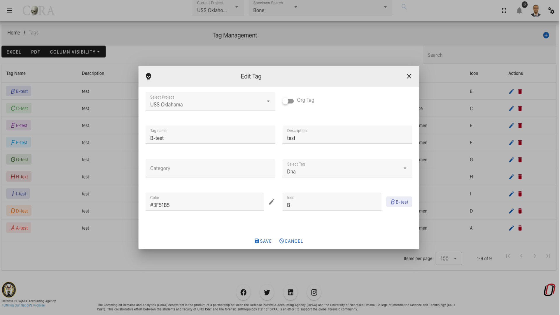
The screen fields are shown below. Fields in bold are required.
| Attributes | Data Type | Size | Validation Rule | Required/Optional |
|---|---|---|---|---|
| Project | Id | valid option via dropdown | Required (Default current project) | |
| Tag Name | String | 32 chars | contains letters and numbers | Required |
| Description | String | 255 chars | contains alphanumeric | Required |
| Category | String | 32 chars | contains letters and numbers | Optional |
| Type | String | 32 chars | contains letters and numbers | Optional |
| Color | String | 32 chars | color hex number | Optional |
| Icon | String | 32 chars | mdi icon (see material design icon codes) | Optional |
Org Profile
CoRA has a very powerful and flexible design which allows every organization to customize how they would like to use CoRA for their projects. The Org Profile screen is where you manage these settings. The information here is organized within tabs, each of these tabs is discussed below.
About
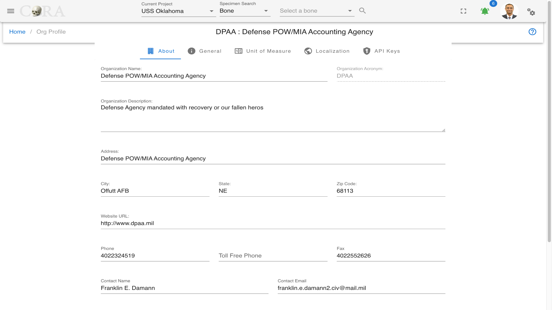
In the About tab the org administrator can edit the Organization Name, Description, Address, Website URL, Phone, Fax, Contact Name, Contact Email, GeoLatitude and GeoLongitude
General
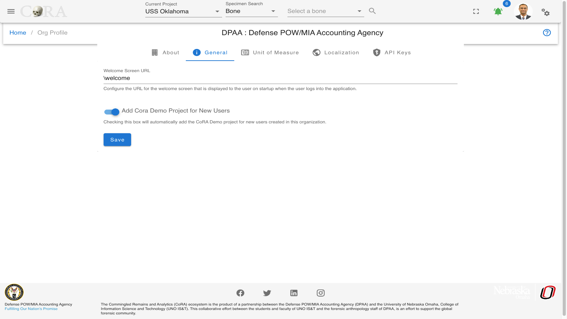
In the General tab the org administrator can configure the URL for the welcome screen that is displayed to the user on startup when the user logs into the application and turn on a switch to automatically add the CoRA Demo project for new users created in their organization.
Unit of Measure
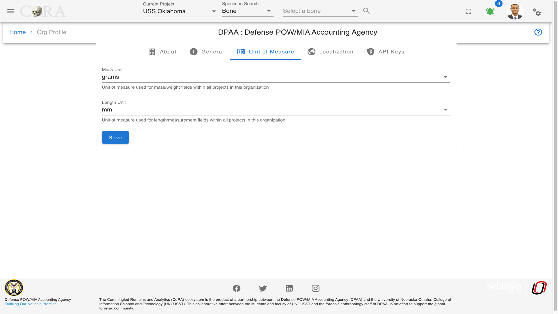
In the Unit of Measure tab the org administrator can configure the unit of measure used for mass/weight and length/measurement fields within all projects in their organization.
- mass/weight, valid values are grams and ounces
- length/measurement, valid values are mm, cm and inches
Localization
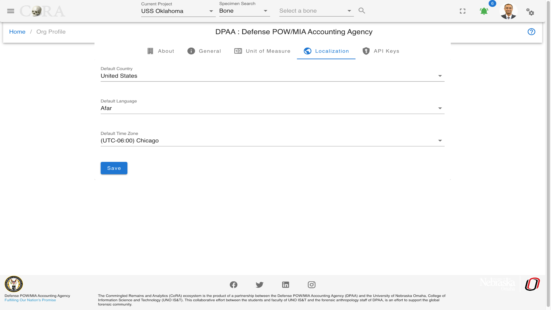
In the Localization tab the org administrator can configure to set the default County, Language and Timezone for all new users created in their organization.
API Keys
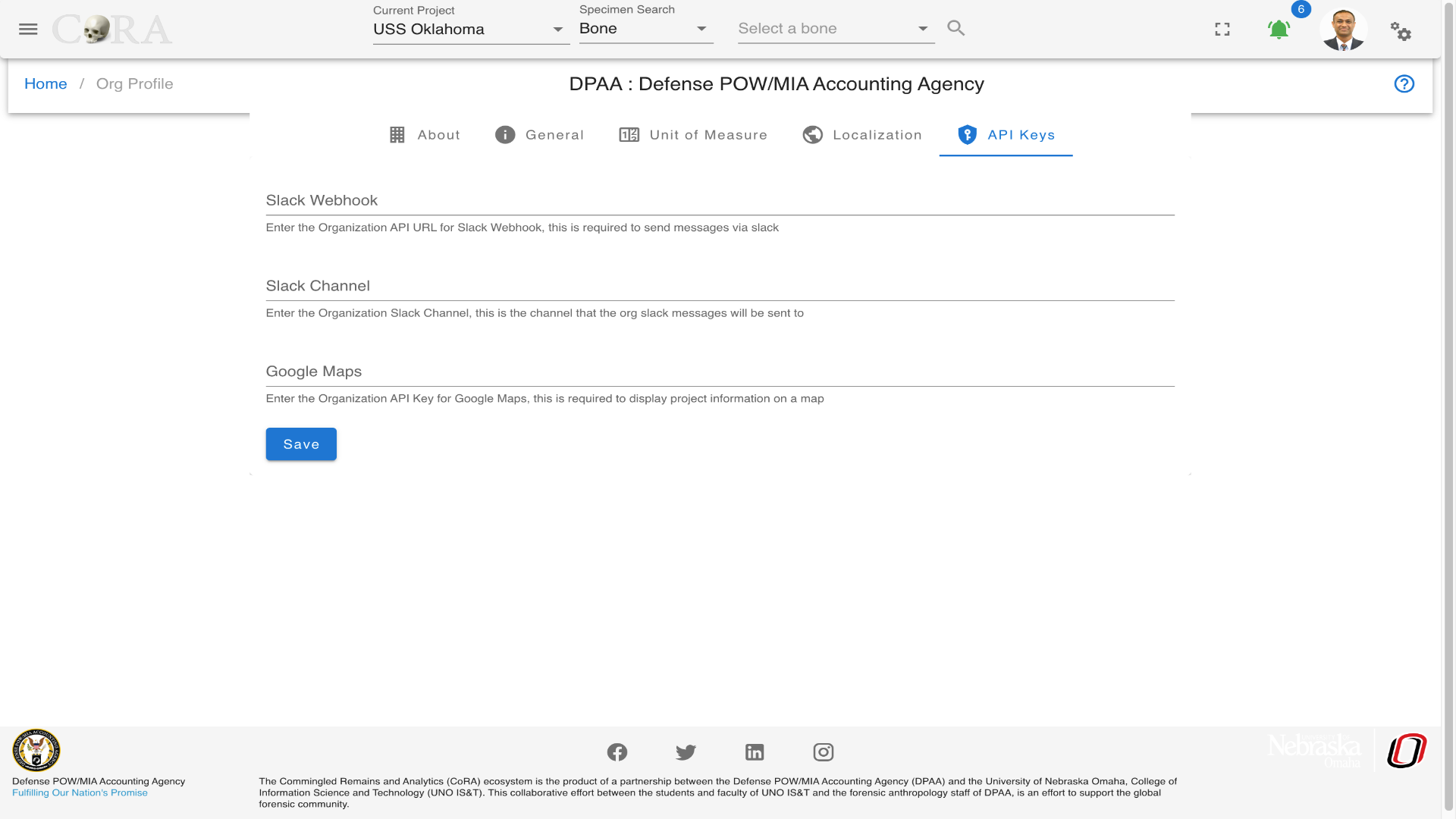
In the API Keys tab the org administrator can configure the following for their organization
- Slack Webhook API URL, this is required to send messages via slack.
- Slack Channel, this is the channel that the organization slack messages will be sent to.
- Google Maps API Key, this is required to display project location information on a map.
User Roles Permissions
The CoRA application's authorization is structured around the concept of user, roles and permissions. What does this mean for you? CoRA was designed with security and traceability in mind to handle both Authentication and Authorization within the application. Each User within the organization has a role and these roles have permissions assigned to them. The roles can be that of Anthropologist, DNA analyst, Isotope Analyst, Manager, etc. Each model or resources within CoRA such as Specimen, DNA, Isotope, Missing Person, etc has browse (list), read, edit, add (create) and delete permissions. Each role has a permission set that allows the user with that role to access specific functionality within CoRA. The entity-relationship diagram below shows this relationship.
erDiagram
  USER ||--o{ ROLE : has
  USER {
    string name
    id role
  }
  ROLE ||--|{ PERMISSION : assignedTo
  ROLE {
    string name
    string description
  }
  PERMISSION {
    string ability
  }
User
Users in CoRA belong to a org and user accounts are created and typically assigned to projects by the org administrator. Anyone who uses CoRA must have a user account and must be assigned a role (such as org administrator, anthropologist, dna analyst, isotope analyst, dentist, historian, etc). Each role is assigned a set of permissions that provides a specific level of authorization to features within CoRA. The users are responsible for managing and updating their user profile which are attributes that control user settings within CoRA.
Roles
Roles in CoRA is a container that holds a set of permissions. In CoRA permissions are assigned to a role which is done by the system.
Roles Table
Following is a list of roles within CoRA.
- Org Administrator
- Manager
- Anthropologist
- Anthropologist - Project Lead
- DNA Analyst
- Isotope Analyst
- Historian
- Dentist
- Intern
- Missing Persons Administrator
- Missing Persons Case Manager
Tip
The org administrator role should be restricted to one user within your organization.
Permissions
Permissions in CoRA are set at the model or resource level. Each model or resources within CoRA such as Specimen, DNA, Isotope, Missing Person, etc has browse (list), read, edit, add (create) and delete permissions. Each role has a permission set that allows the user with that role the ability to access specific functionality within CoRA.
User Profile
CoRA has a very powerful and flexible design which allows every user to customize how they would like to use CoRA for their projects. Creating a good and friendly user experience is what CoRA strives for. Users can navigate to the user profile by clicking on the avatar icon on the top right corner. The User Profile screen is where you manage these settings. The information here is organized within tabs, each of these tabs is discussed below.
About Profile
In the About tab the user can view their current details and can edit the Name, Cell Phone, Alternative Phone, Slack Channel. The Email and the Organization name are readonly.

General
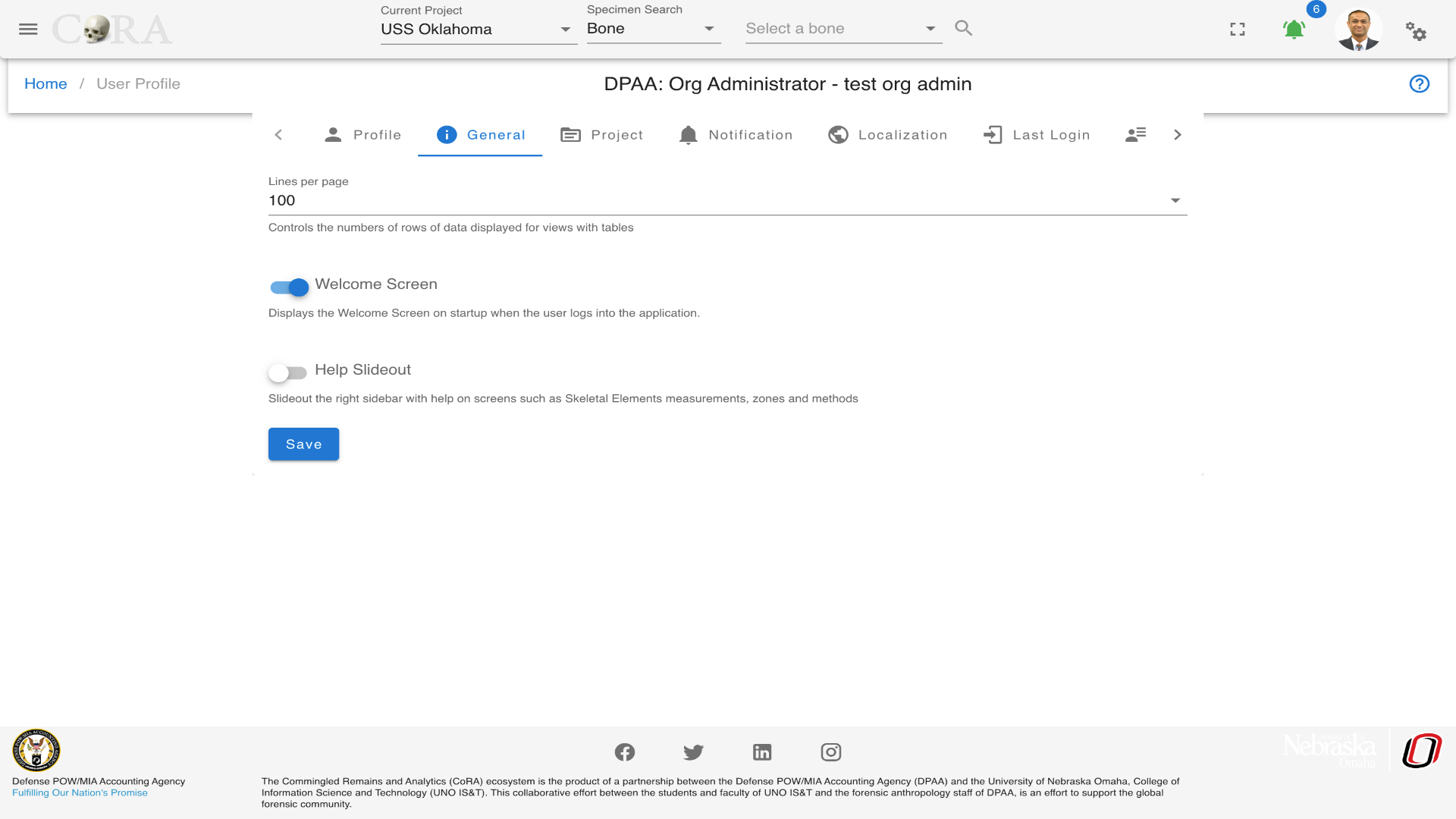
In the General tab the user can update the following
- Lines per page, this will control the numbers of rows to display in data tables within CoRA.
- Welcome Screen, user can choose to display the Welcome Screen on startup when the user logs into the application.
- Help Slideout, user can choose to have help slide out the right sidebar with help on screens such as Specimen measurements, zones and methods.
Project
In the Projects tab the user can update the following within expansion panels.
- Project:
- User can set the default project to use when the user logs into the application.
- Specimen:
- User can set the accession, provenance1 , provenance2 number that will be auto-populated on New Specimen screen.
- The MRU List specimen is the number of Most Recently Used/Accessed (MRU List) Specimens to keep track of.
- User can set a page direct to any Specimen association module after the creation of a new Specimen.
- DNA
- The user can set the lab to be auto-populated on the DNA association screen for Specimen.
- Users can add a configurable default search option to use for quick search.
- The DNA method will be auto-populated on Y-STR, auSTR DNA associations for Specimens based on the selections in the tab.
- Also the user can choose to select an option that will use older DNA sample record information if a new DNA sample record exists but has NULL values.
- Search:
- User can set a default search option.
- User can an save the last used Search By criteria and the search will be defaulted to this saved Search By criteria.
- User can choose to open the Specimen screen in a new tab via the Search results screen.
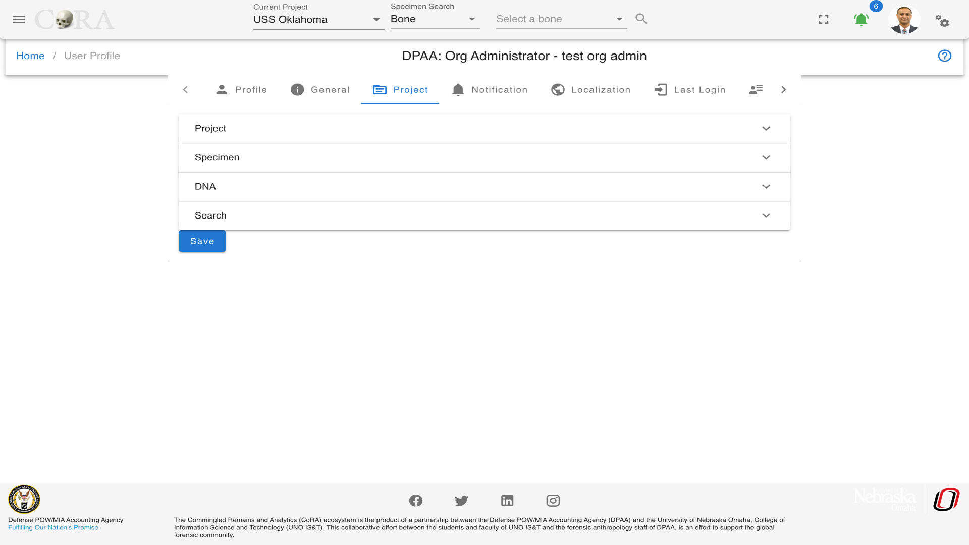
Notification
In the Notification tab the user can choose to receive a notification when 1. Either an export or import job is completed that was initiated by that user. 2. When a specimen has been marked as reviewed, 3. When changes are made to the DPAA Priority field in Missing Persons records. 4. User can select which methods for notification they want to use. The notification can be through Email, SMS, or Slack.
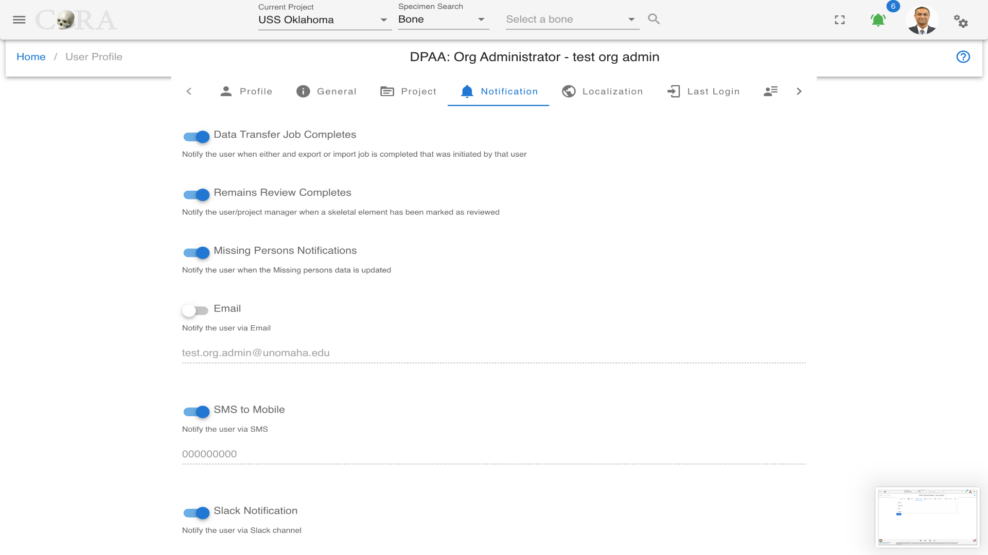
Localization
In the Localization tab the user can update their default County, Language and Timezone.
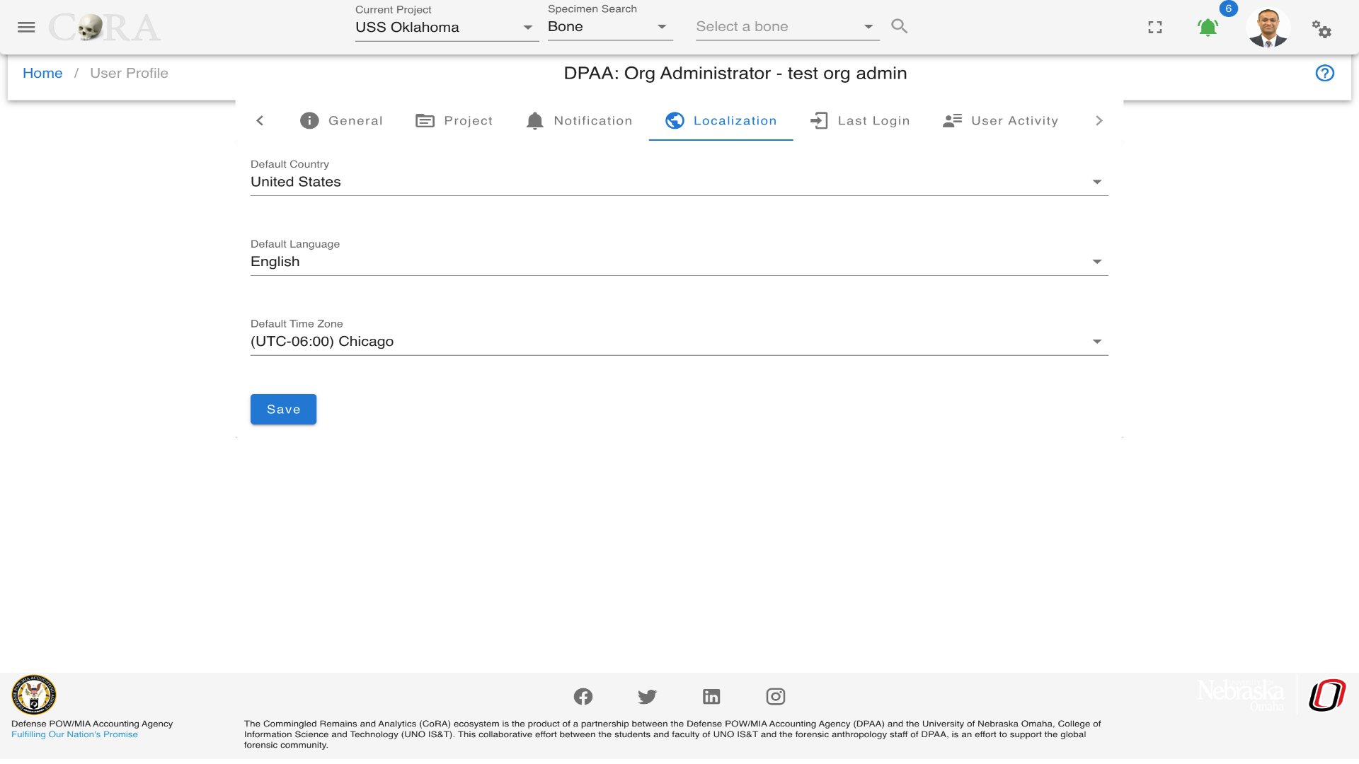
Last Login
In the Last Login tab the user can view information such as last login time, Device, Total Number of logins, IP address and Password last changed.
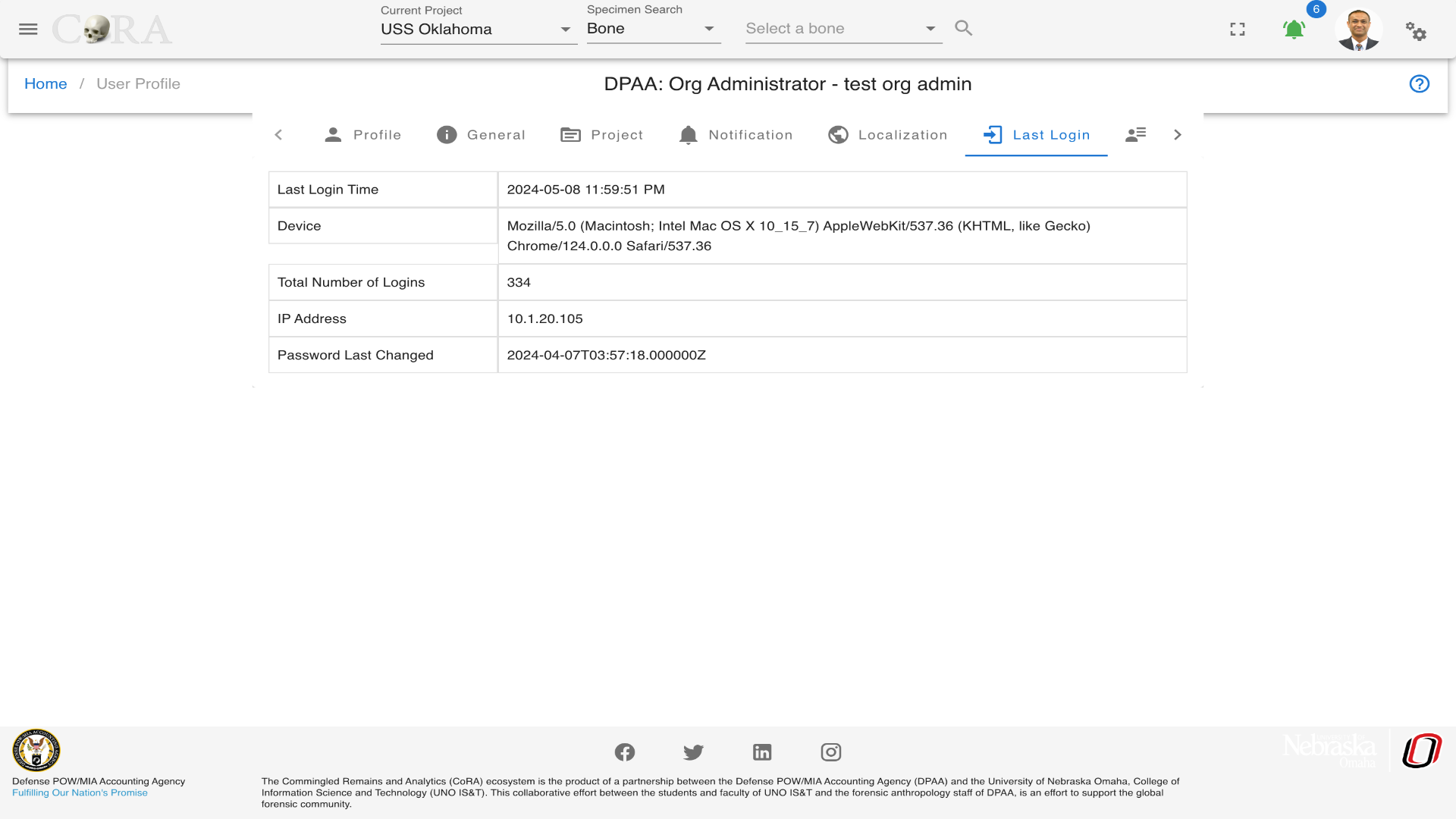
User Activity
In the User Activity tab the user can view the user activity feed for specimens as a table with columns such as Key, Name, Side, Completeness and Updated At details. Also there is the user activity feed table for DNA with the fields such as key, Mito sequence Number, Mito sequence subgroup and Update at columns with details.
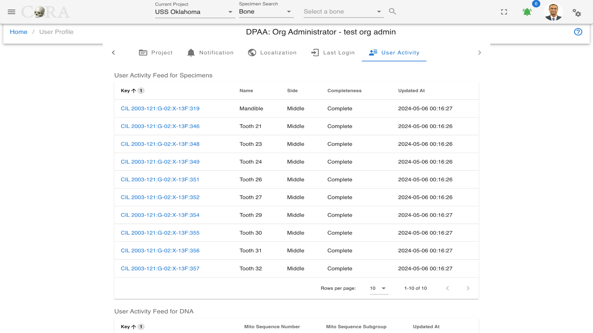
User Notifications
The User Notifications feature keeps users informed about important updates, activities, or system events related to their work in CoRA. Notifications appear in two areas 1. The popup panel 2. The Notifications Management page.
Popup Notifications
Users can access notifications by clicking the bell icon beside their profile avatar at the top-right corner of the screen.
When selected, a popup appears showing a summary of recent notifications.
Within this popup:
- Unread Notifications Count – Displays the total number of unread notifications for the user.
- Type – The category of the notification, such as System, User, or Project.
- Details – A short message summarizing the event or action.
- Actions –
- View All (eye icon): Opens the Notifications Management page.
- Mark All as Read (checkmark icon): Marks all displayed notifications as read.
If there are no notifications available, the message “No data available” is displayed.
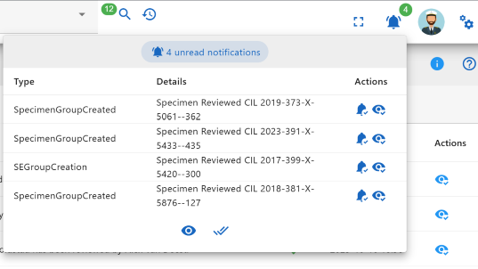
Notifications Management
Clicking the eye icon from the popup opens the Notifications Management screen.
This page lists all notifications for the user, allowing them to review, filter, or manage notifications as needed.
Fields in this table include:
- Type – Identifies the type of notification (for example, System, User, or Project).
- Description – Provides a short summary of the event or update.
- Details – Displays additional information related to the notification, such as specimen ID or user activity.
- Read – Indicates whether the notification has been viewed.
- Created At – Shows the date and time the notification was generated.
- Actions – Allows the user to mark a notification as read or perform other related actions.
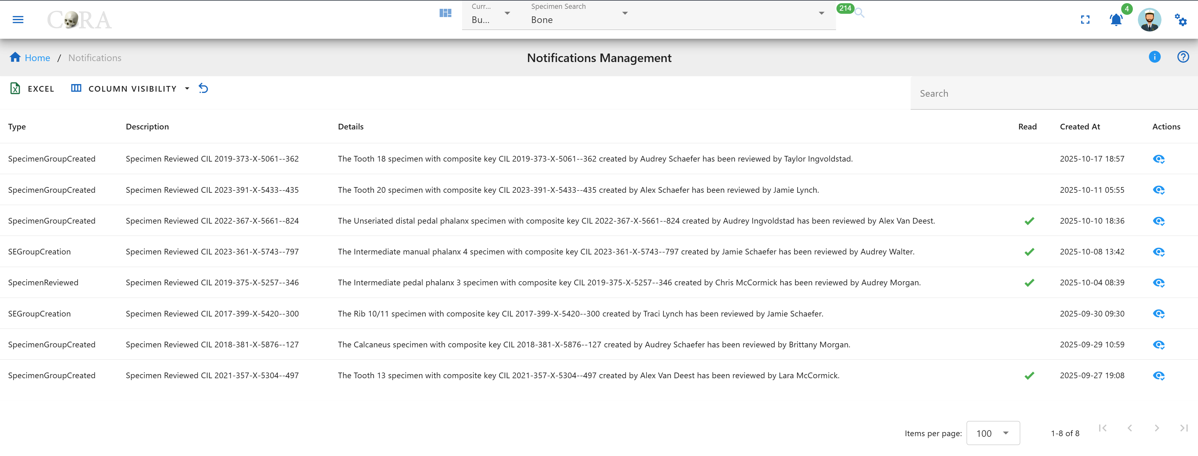
At the bottom of the page, the Items per page dropdown lets users control how many notifications are visible at once.
If there are no notifications to display, the message “No data available” will appear.
User Authentication
This section shows you how to sign in to CoRA and what to expect along the way—whether everything works smoothly or you need to take an extra step. We'll also explain the security checks that protect your access in simple terms.
Why Authentication Matters
Authentication is the front door that keeps sensitive data safe. CoRA follows security best practices: only authorized users with the right credentials can sign in, suspicious activity (like repeated wrong passwords) is blocked, and passwords regularly expire to keep accounts secure.
How This Guide is Organized
How to Log In — the steps from clicking Login to reaching the Home page
What You Might See — explanations of any messages that appear and what to do about them
Security Notes — simple explanations of the security checks happening when you sign in
How to Log In
Step 1: Go to the Login Page
Click the LOGIN button in the top right corner of your screen.
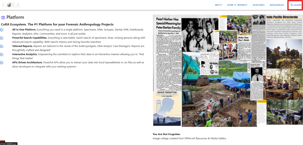
Step 2: Enter Your Credentials
Type in your email address and password.
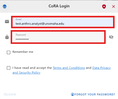
Step 3: Accept the Terms and Log In
Check the boxes to agree to the Terms and Conditions and Data Privacy and Security Policy. Then click Login.
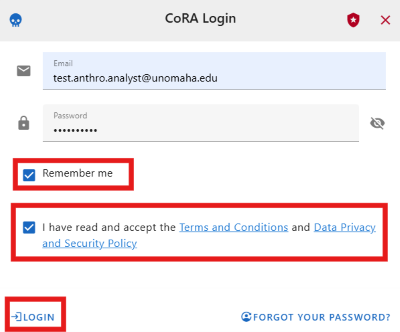
Step 4: Access CoRA
If your email and password are correct and your account is active, you'll be signed in and taken to the home page.
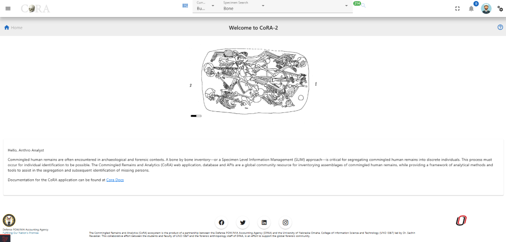
First-Time Login
If this is your first time logging in, you'll need to create your own password.
Step 1: Go to the Login Page
Click the LOGIN button in the top right corner.
Step 2: Enter Your Temporary Credentials
Your administrator will provide you with a temporary email address and password. Enter those credentials.
Step 3: Accept the Terms and Log In
Check the boxes to agree to the Terms and Conditions and Data Privacy and Security Policy. Then click Login.
Step 4: Create Your New Password
You'll be prompted to change your password immediately. Enter your temporary password, then type your new password twice to confirm it.
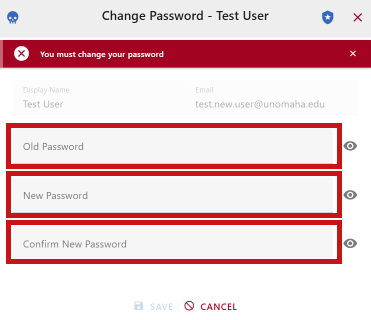
Step 5: Log In with Your New Password
Enter your email address and the new password you just created.
Step 6: Access CoRA
You'll now be signed in and taken to the home page.
Common Login Issues and What They Mean
Wrong Email or Password
If you enter an incorrect email address or password, you'll see this message: "Invalid credentials. Please try again."
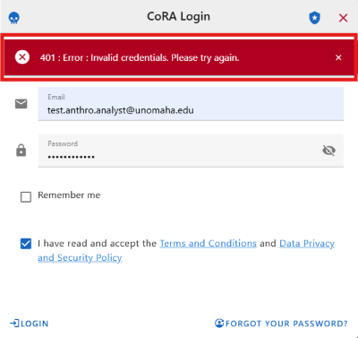
What to do: Double-check your email and password, then try again.
Inactive Account
If your account has been inactive for more than 60 days or was disabled by an administrator, you'll see: "Your user account has been inactive beyond 60 days. Please contact your System Administrator."
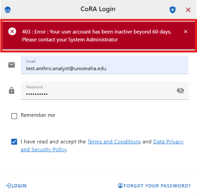
What to do: Contact your system administrator to reactivate your account.
Password About to Expire
Passwords expire every 60 days for security. Starting 10 days before expiration, you'll see a reminder to reset your password when you log in.
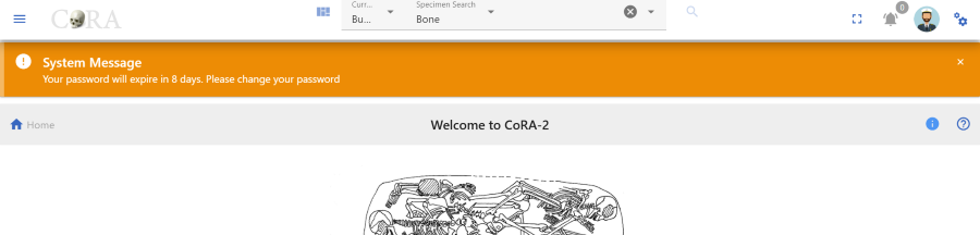
What to do: Follow the prompts to create a new password before the 60 days are up.
Password Has Expired
If your password has expired (after 60 days), you'll still be able to log in, but you'll be required to change it before you can do anything else in CoRA.
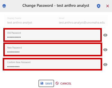
Important: Your new password cannot be the same as any of your last three passwords.
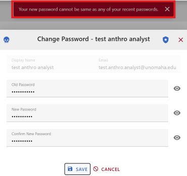
What to do: Create a new, unique password.
Too Many Failed Login Attempts
If you enter the wrong credentials five times in a row, your account will be temporarily locked for security reasons.
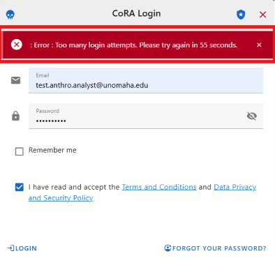
What to do: Wait a few minutes, then try logging in again. If you've forgotten your password, contact your administrator.
Modules
Modules
Design Methodology
CoRA is built on an architectural framework consisting of various components including some core components such as the navigational and authentication components. The rest of the site is logically structured around modules, which are plugged into the framework and they interact with each other.
Modules
CoRA is structured around some core modules such as Specimens, DNA, Isotopes, Dental, Missing Persons and Individuals modules. Each of these modules is described in more detail below.
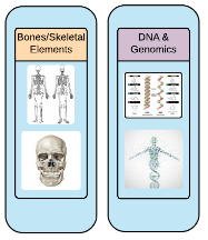
Specimens
DNA
Isotopes
Dental
Missing Persons
Individual
An individual is a collection of specimens that the forensic anthropologist believe should go together and belong to an unknown individual. The selection of specimens that go together is done in blind so as to not introduce any bias towards the segregation process.
Specimens or Skeletal Elements
Specimen are individual human remains which can be categorized. Many of the modules on the site are focused on specimens and their association details such as Biological Profile, DNA Profile, Measurements, Zones, Articulation, Pair Matching, Refits, Morphology, Pathology, Trauma, Taphonomy, etc. This section will explore navigating the specimens and their associations screen related characteristics.
The Specimen navigation menu includes:
- New Specimen
- New via Bone Group
- Associate Bone Groups
- Assign Specimens to Bone Group
- Advanced Search
Specimen Navigation
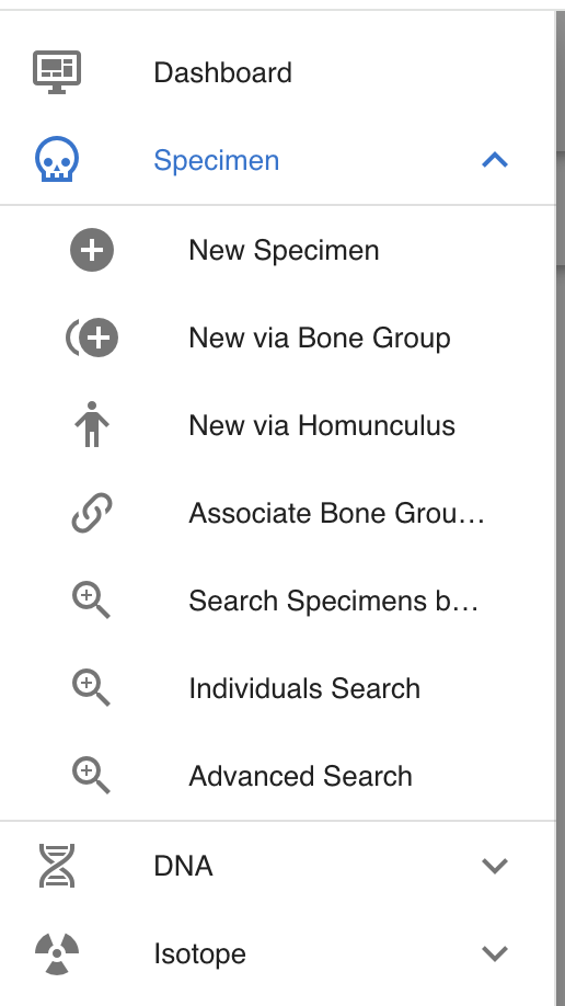
On the left side bar - you can access the main options for specimens. For Report Dashboard - please see the Reports documentation.
Creating Specimens
You can create a new specimen in multiple ways. For example you can create a a single specimen or multiple specimens belonging to a bone group such as Arm, Shoulder, Vertebral Column, Hand, Feet, etc. In the future we plan to include specimen creation via a Homunculus. I know I'm getting ahead of myself but that is on our dream list.
Single Specimen
To create a new specimen navigate to the Left Sidebar Menu -> Specimen -> New Specimen. You will be taken to the new specimen screen as shown below.
The screen fields are shown below. Fields in bold are required.
| Attributes | Data Type | Size | Validation Rule | Required/Optional |
|---|---|---|---|---|
| Accession | String | 32 chars | Can only contain letters, numbers, dash and space and should have min 3 chars | Required |
| Provenance1 | String | 32 chars | Can only contain letters, numbers, dash and space | Optional |
| Provenance2 | String | 32 chars | Can only contain letters, numbers, dash and space | Optional |
| Designator | Alphanumeric | 32 chars | Can only contain letters and numbers | Required |
| External ID | String | 32 chars | Can only contain numbers and decimals | Optional |
| Bone | Id | id | valid bones via dropdown | Required |
| Side | String | 8 chars | valid sides via dropdown (Left, Right, Middle, Unsided) | Required |
| Completeness | String | 16 chars | valid completeness via dropdown (Complete, Incomplete) | Required |
Once these details are filled and the user can either select 'SAVE AND EDIT' or 'SAVE AND ADD'. If the user selects 'SAVE AND EDIT', a new specimen with an appropriate id is generated and the user is navigated to the below screen. The screen is in View state.
- Edit button enables the user to edit the specimen.
- The Kebab menu button consists of DNA profile, Isotope Analysis, Zone Classification, Taphonomy, all specimen associations and pathology, and Review.
To edit a specimen, you can search for it using the advanced search feature under specimen menu or the search function available on the home page.
Edit a specimen via the home page search
 Edit specimen via Specimen→Advanced Search
The screen fields are shown below. Fields in bold are required.
| Attributes | Data Type | Size | Validation Rule | Required/Optional |
|---|---|---|---|---|
| Accession | String | 32 chars | Can only contain letters, numbers, dash and space and should have min 3 chars | Required |
| Provenance1 | String | 32 chars | Can only contain letters, numbers, dash and space | Optional |
| Provenance2 | String | 32 chars | Can only contain letters, numbers, dash and space | Optional |
| Designator | Alphanumeric | 32 chars | Can only contain letters and numbers | Required |
| External ID | Alphanumeric | 32 chars | Can only contain numbers and decimals | Required |
| Bone | Id | id | valid bones via dropdown | Required |
| Side | String | 8 chars | valid sides via dropdown (Left, Right, Middle, Unsided) | Required |
| Completeness | String | 16 chars | valid completeness via dropdown (Complete, Incomplete) | Required |
| Measured | Boolean | true/false toggle | Optional | |
| DNA Sampled | Boolean | true/false toggle | Optional | |
| Isotope Sampled | Boolean | true/false toggle | Optional | |
| Inventory Completed | Boolean | true/false toggle | Optional | |
| Reviewed | Boolean | true/false toggle | Optional | |
| CT Scanned | Boolean | true/false toggle | Optional | |
| X-ray Scanned | Boolean | true/false toggle | Optional | |
| 3D Scanned | Boolean | true/false toggle | Optional | |
| Individual Number | String | 32 chars | can only contain letters, numbers, dash and space | Optional |
| Remain Status | String | 16 chars | valid sides via dropdown (In Lab, Released) | Optional |
Click "Save" When you are done making changes.
A specimen can be deleted by clicking on the delete icon and then confirming the deletion in the pop-up.
Multiple via Bone Group
To create a multiple specimens via bone group - navigate to the Left Sidebar Menu -> Specimen -> New via Bone Group. You will be taken to the new specimens via bone group screen. Here you can create multiple specimens that belong to the same bone group.
Tip
This is the preferred way to create multiple specimens within a bone group as CoRA will automatically create articulation relationship amongst them. You can also apply Pathology, Trauma and Taphonomy to these specimens at the time of creation simplifying and speeding up the data entry process.
The fields to create a new bone group are:
- Bone Group
- Grouping
- Bones
- Side (defaulted to 'Left')
- Completeness (defaulted to 'Complete')
- Accession
- Accession Number
- Provenance 1
- Provenance 2
- Designator
- Pathology
- Traumas
- Pathologies
- Taphonomies
The bolded fields are required. Once you have created a new bone group, you can edit the fields and click "Save" to update the bone group.
| Attributes | Data Type | Size | Validation Rule | Required/Optional |
|---|---|---|---|---|
| Bone Group | String | 64 chars | can only contain letters | Required |
| Bone Group Id | String | 64 chars | valid UUID, auto generated | Required |
| Side | String | 8 chars | valid sides via dropdown (Left, Right, Middle, Unsided) | Required |
| Completeness | String | 16 chars | valid completeness via dropdown (Complete, Incomplete) | Required |
| Accession | String | 32 chars | can only contain letters, numbers, dash and space and should have min 3 chars | Required |
| Provenance1 | String | 32 chars | can only contain letters, numbers, dash and space | Optional |
| Provenance2 | String | 32 chars | can only contain letters, numbers, dash and space | Optional |
| Starting Designator | Alphanumeric | 32 chars | can only contain letters and numbers | Required |
| Bone | Id | id | valid bones via dropdown | Required |
Once you have created a new bone group, you can edit the fields and click "Save" to update the bone group.
Tip
When creating specimens via bone groups, you only have to specify the starting designator and CoRA will automatically create the specimens with that starting designator and increment it for subsequent specimens within the bone group.
Multiple via Homunculus
To create a multiple specimens via homunculus - click the "New via homunculus" link on the Specimens left navigation bar. You will be taken to the new specimens via homunculus screen.
Warning
This is an experimental feature and is work in progress. We will keep you posted when this feature is available.
Specimen Actions or Details
The screenshot below shows the Actions or Details menu for the selected specimen. Here you can enter association data for the specimen. Each of the Action or Details menu option is explained in the following section.
DNA Status Indicators in Specimen List
When viewing specimen lists or search results, you'll see color-coded DNA status indicator bars that provide a quick visual overview of DNA profile completion for each specimen. These progress indicators help you track data entry completion across the three main DNA testing categories.
Understanding the DNA Status Bars
Each specimen displays four DNA indicator sections from left to right:
- DNA Sample Count - Shows the total number of DNA samples for the specimen
- Green bar: DNA sample(s) exist
- Orange bar: No DNA samples
-
Displays the number of samples and their sample numbers
-
Mito (Mitochondrial DNA) - Tracks completion of mitochondrial DNA fields
- Green bar: At least one Mito field is completed
- Orange bar: No Mito fields completed
- Displays a ratio showing completed fields out of total available fields
-
Shows Mito sequence number, sequence subgroup, sequence similar and field count when available
-
au-STR (Autosomal DNA) - Tracks completion of autosomal DNA fields
- Green bar: At least one au-STR field is completed
- Orange bar: No au-STR fields completed
- Displays a ratio showing completed fields out of total available fields
-
Shows au-STR sequence number, sequence subgroup, sequence similar and field count when available
-
y-STR (Y-Chromosome DNA) - Tracks completion of Y-chromosome DNA fields
- Green bar: At least one y-STR field is completed
- Orange bar: No y-STR fields completed
- Displays a ratio showing completed fields out of total available fields
- Shows y-STR sequence number, sequence subgroup, sequence similar and field count when available
Tip
Click on any DNA status indicator card to navigate directly to the corresponding DNA profile tab (Mito, au-STR, or y-STR) to complete or review the data fields. The color-coding provides instant feedback on which DNA profiles need attention.
Biological Profile
The Biological Profile is where you can record the various methods and method features for method type Age, Ancestry, Sex, and Stature. CoRA's intellisense engine will automatically provide you the available methods for each method type which are currently registered in CoRA. The user can add, edit or delete a method.
Age
Sex
Ancestry
Stature
Warning
This section needs to be documented
DNA Profile
The DNA Profile screen displays the following elements about a bone:
- DNA Sample Number
- Lab
- External Case #
- BTB Request Date
- BTB Results Date
- Disposition
- Sample Condition
- Weight Sample Remaining
On this screen, you can also view the "Mito", "auSTR", and "Y-STR" forms and navigate by clicking the form name or by clicking the Next button.
Isotope Analysis
The 'Create Isotope' section allows to create a isotope for the given bone. This section has the following elements. - Lab - External Case # - Isotope Sample Number
After you create the Isotope, you will receive the "success" message. By selecting the sample number, the Isotope screen pops up. Click on the Edit button to edit the information under each section.Click on the Save button under each section saves the information and navigates the user to the next section of information. All the updated information can be saved at once by clicking on the ‘Save All’ button.
Taphonomy
The Taphonomies section allows you to view Taphonomies for the given bone. To add Taphonomy, click the pencil icon to edit and select Taphonomies. Click the Save icon to save the changes.
Zonal Classification
The Zones pane displays various zones of the bone. For example below are the following zones about the Cervical Vertebra:
- Body
- Right Transverse Process
- Left Transverse Process
- Spinous Process
These fields are read only - to edit then click the pencil icon. Multiple zones can be selected. All the listed Zones can be selected or deselected by clicking the ‘Select all’ check box. Click the save icon to save the changes.
Measurements
The measurements pane displays various measurements of the given bone. Only the specimens associated with a bone that is measured will have measurements for that bone. Bones associated with a specimen that are not measured will not have any measurements. The measurements generally vary from one bone to another and following are the measurements for a given bone Femur:
- Fem_01 Maximum Length
- Fem_02 Bicondylar Length
- Fem_03 Epicondylar Breadth
- Fem_04 Maximum Head Diameter
- Fem_05 Medial-Lateral (Transverse) Subtrochanteric Diameter
- Fem_06 Anterior-Posterior (Sagittal) Subtrochanteric Diameter
- Fem_07 Anterior-Posterior (Sagittal) Midshaft Diameter
- Fem_08 Medial-Lateral (Transverse) Midshaft Diameter
- Fem_09 Maximum Midshaft Diameter of the Femur
- Fem_10 Minimum Midshaft Diameter of the Femur
- Fem_11 Midshaft Circumference
- Fem_12 Maximum Anterio-posterior Length of the Lateral Condyle
- Fem_13 Maximum Anterio-posterior Length of the Medial Condyle
- Fem_14 Minimum Anterior-Posterior Diameter of the Diaphysis
- Fem_15 Minimum Medial-Lateral Diameter of the Diaphysis
- Fem_16 Minimum Superior-Inferior Neck Diameter
- Fem_17 Maximum Diameter along the Linea Aspera
- Fem_18 Upper Breadth of Femur
- Fem_19 Lateral Condyle Height
These fields are read only - to edit, click the pencil icon. the minimum value, threshold limit and maximum limit are indicated to the user through the alerts. Click the save icon to save the changes or ‘Undo’ icon to undo all the changes made. The blue badge on top of the bone name indicates the number of measurements filled out of the total number of available measurements for that particular bone. The pane can be expanded or collapsed by clicking on the arrow icon.
Associations
There are four types of associations. Process of adding each association is shown below. After the association is added, refresh the page to see the Details button updated. The details button opens a data table of all available associations under that specimen.
Pair
Articulations
Refits
Morphology
Pathology, Anomaly & Trauma
Pathology, Trauma and Anomaly can be accessed on one screen as different tabs. The user can create a new item by clicking on the create button.
Pathology
Anomaly
Trauma
Specimen Review
The review tab is a pane which displays all other sub reports in one area. All reports are editable in the pane. For information on individual reports - see their detailed documentation.
Specimen Bulk Edit
Several specimen fields can be bulk-edited. To bulk edit, select multiple specimens by clicking in the boxes next to the specimens you want to edit, click on the Actions tab, and then select Batch Edit.
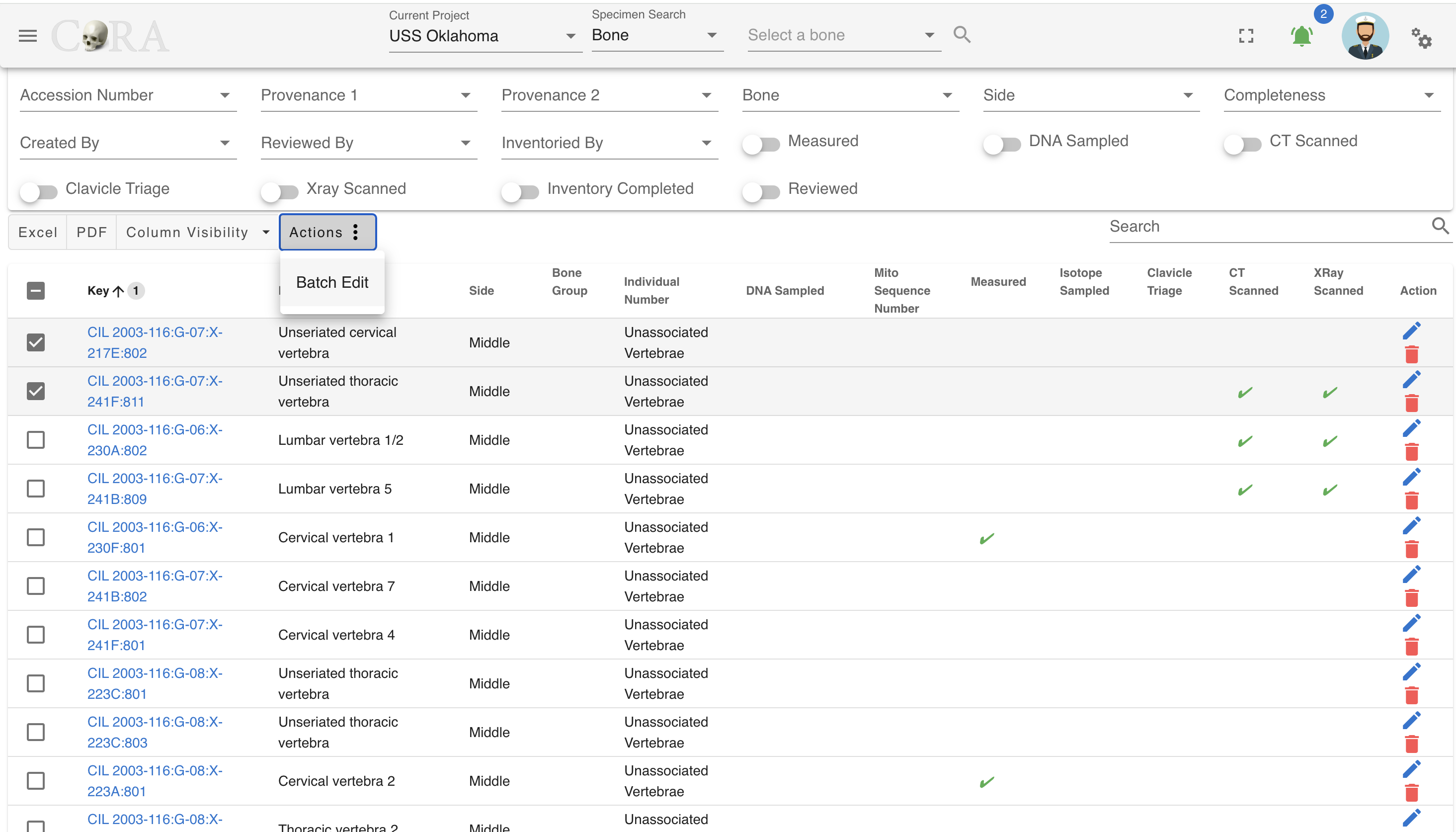
In the popup, select the changes you wish to make. When you mark a specimen as scanned, completed, or reviewed, the date for the change is auto-filled to the current date.
If the remains are marked as in the lab, there is no corresponding date.
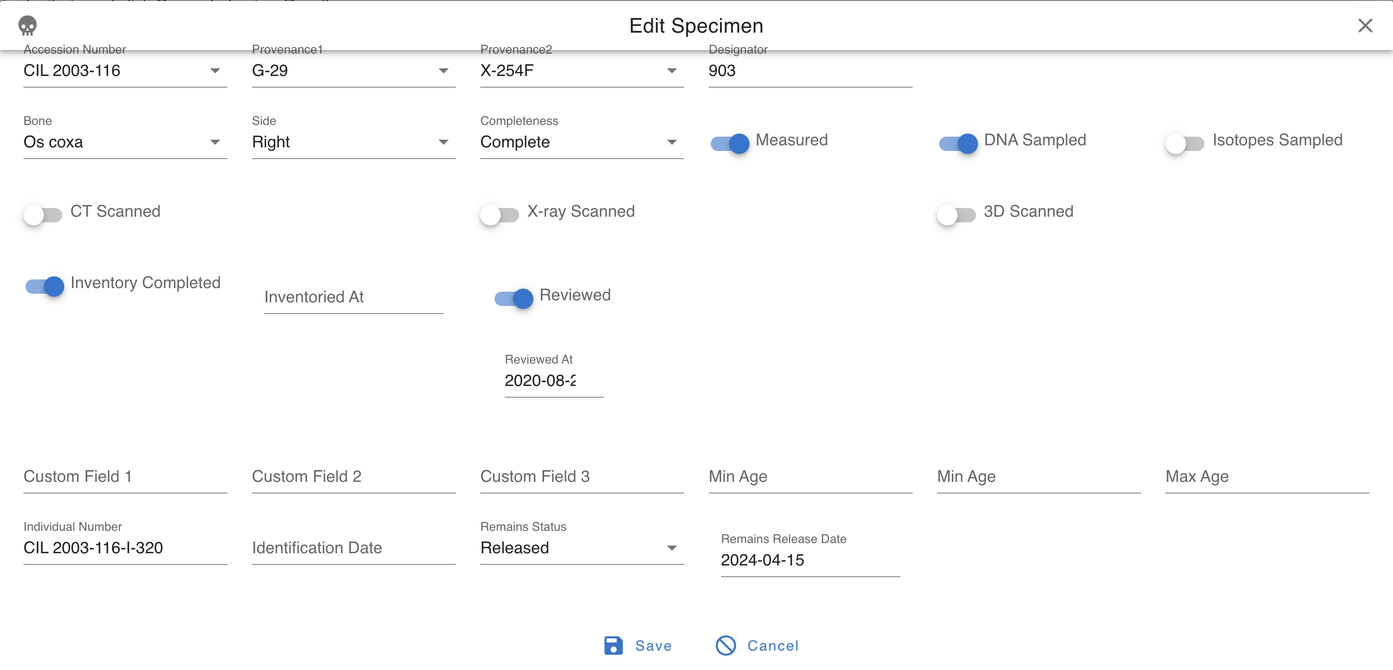
If the remains are marked as released, there is a date field.
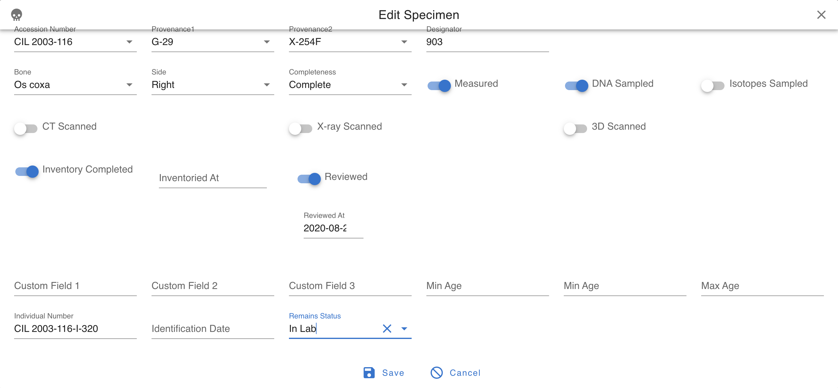
Associate Specimen By Bone Group
The Associate Specimen By Bone Group feature allows users to pair and manage bone groups interactively. This functionality is enhanced with drag-and-drop capabilities for intuitive association.
Steps to Associate Specimens by Bone Group
1. Access the Feature:
Navigate to the left sidebar menu and select Specimens > Associate Bone Groups.

2. Filter Bone Groups:
- Use the dropdown menus to filter by:
- Bone Group
- Side (Left, Right, Unsided)
- Click the Load Groups button to display matching bone groups.
3. Associate Bone Groups:
- Select a bone group from the left column (e.g., "Right Bone Groups").
- Select or drag to the corresponding bone group from the right column (e.g., "Opposite Side").
4. Save or Cancel:
- To save the associations, click the Associate Groups button.
- To cancel the operation, click the Cancel button.
Key Features
- Dynamic Filtering: Quickly locate relevant bone groups using filters for Bone Group and Side.
- Column-Based Selection: Select bone groups from separate columns for pairing.
- Association Confirmation: Use the "Associate Groups" button to confirm pairings.
- Real-Time Updates: Changes are reflected immediately upon saving.
Example Workflow
- Filter bone groups by "Hand" and "Right".
- Click Load Groups to display matching bone groups.
- Select a bone group from the "Right Bone Groups" column.
- Select or drag to the corresponding bone group from the "Opposite Side" column.
- Click the Associate Groups button to confirm the pairing.
Assign Specimen to Bone Group
The Assign Specimen to Bone Group feature allows users to associate one or more specimens with a specific bone group. This functionality is particularly useful for organizing specimens into predefined categories such as Arm, Shoulder, Vertebral Column, etc.
Steps to Assign Specimens to a Bone Group
1. Access the Feature:
Navigate to the left sidebar menu and select Specimens > Assign Specimens to Bone Group.

2. Select Specimen:
- If you have pre-selected specimens, they will appear in the "Selected Specimens" section.
- To load all project specimens, click the Load All button.
3. Apply Filters (Optional):
- Use the available filters to refine the list of specimens based on:
- Accession
- Provenance 1
- Provenance 2
- Bone
- Bone Group
- Individual Number
- Side
- Completeness
4. Select Bone Group:
- Choose the target bone group from the dropdown menu to which the specimens will be assigned.
5. Drag and Drop Specimens:
- Select the desired specimens from the list.
- Drag and drop the specimens into the bone group selection area.
6. Save or Cancel:
- Select the reasons for each assignment.
- Then to save the assignments, click the Save button.
- To cancel the entire process, click the Cancel button.
- You can also delete individual specimens from the selection by clicking the X icon within the card to them.
Key Features
- Dynamic Specimen List: The list updates based on applied filters, ensuring you only see relevant specimens.
- Bulk Assignment: Assign multiple specimens to a bone group in one action using drag-and-drop functionality.
- Real-Time Updates: Changes are reflected immediately in the project database after saving.
Example Workflow
- Filter specimens by "Accession" and "Bone Group".
- Select all specimens in the filtered list.
- Select the "Hand" bone group from the right-hand dropdown.
- Drag and drop them into the "Hand" bone group selection area.
- Once completed with all selections select the reason for each assignment.
- Click Save to finalize the assignments.
Specimen Search
The easiest way to search for specimens is to use the top search bar in the header. To find out more visit the search documentation
DNA
DNA can be an important step in the identification process of missing persons. If your project chooses to use DNA analysis as part of your identification process then you have come to the right place. Here you will learn more about the DNA module in CoRA. A critical first step is to cut a sample of the specimen for DNA analysis and then assign a sample number to it for tracking purposes and after you get results from your DNA lab you can capture DNA information here to create a DNA Profile for further analysis.
DNA Navigation

Navigate to the Dental section by opening the navigation bar and selecting the Dental dropdown.
Create a DNA Sample
The DNA sample and Profile are associated with a specimen, so you must first choose a specimen for which you want to create a DNA sample for. You can choose a specimen by navigating to the specimen screen from either the specimen search results screen or from any data table row that has a specimen link on it. All search and reports screens have specimen links on them. Simply click these links to navigate to the specimen view/edit screen. Once on the specimen screen you can navigate to the Specimen Action or Details, and then to the DNA Profile menu.
CoRA's intellisense will automatically take you to the Create DNA sample screen, if this is the first DNA sample you are trying to create for this specimen or will take you to the DNA list screen if a DNA Sample was previously created for this specimen. Note you can create multiple DNA samples for a specimen.
Tip
CoRA allows you to create multiple DNA samples for a specimen. If you have multiple dna samples, CoRA will create a Consensus DNA Profile for you with data from the multiple samples. Consensus DNA Profile is a powerful feature of CoRA.

The screen fields are shown below. Fields in bold are required.
| Attributes | Data Type | Size | Validation Rule | Required/Optional |
|---|---|---|---|---|
| Sample Number | Alphanumeric | 8 chars | can only contain letters and numbers | Required |
| Lab | Id | id | valid labs via dropdown setup for the org | Required |
| External Case Number | String | 32 chars | Optional |
Clicking Save will take you to the DNA Profile screen. You can visit the DNA Profile screen once you have received data from your DNA processing lab to enter DNA related data.
DNA List Status Indicators
When viewing the DNA List, you'll see color-coded status indicator bars that provide a quick visual overview of DNA profile completion for each specimen. These progress indicators help you track data entry completion across the three main DNA testing categories.
Understanding the Status Bars
Each DNA sample displays four indicator sections from left to right:
- DNA Sample Count - Shows the total number of DNA samples for the specimen
- Green bar: DNA sample(s) exist
- Orange bar: No DNA samples
-
Displays the number of samples and their sample numbers
-
Mito (Mitochondrial DNA) - Tracks completion of mitochondrial DNA fields
- Green bar: At least one Mito field is completed
- Orange bar: No Mito fields completed
- Displays a ratio showing completed fields out of total available fields
-
Shows Mito sequence number, sequence subgroup,sequence similar and field count when available
-
au-STR (Autosomal DNA) - Tracks completion of autosomal DNA fields
- Green bar: At least one au-STR field is completed
- Orange bar: No au-STR fields completed
- Displays a ratio showing completed fields out of total available fields
-
Shows au-STR sequence number, sequence subgroup, sequence similar and field count when available
-
y-STR (Y-Chromosome DNA) - Tracks completion of Y-chromosome DNA fields
- Green bar: At least one y-STR field is completed
- Orange bar: No y-STR fields completed
- Displays a ratio showing completed fields out of total available fields
- Shows y-STR sequence number, sequence subgroup, sequence similar and field count when available
Tip
Click on any status indicator card to navigate directly to the corresponding DNA profile tab (Mito, au-STR, or y-STR) to complete or review the data fields. The color-coding provides instant feedback on which DNA profiles need attention.
Edit DNA Profile
Specimens which have had a DNA sample successfully created will have an associated DNA Profile. The DNA profile contains all the relevant DNA attributes and are editable via action (user must have appropriate role and permissions).
You can visit the DNA Profile screen once you have received data from your DNA processing lab to enter DNA related data to build the DNA Profile for the specimen. On this screen click the pencil icon on the top right corner to edit the DNA profile.
The screen fields are shown below. Fields in bold are required.
| Attributes | Data Type | Size | Validation Rule | Required/Optional |
|---|---|---|---|---|
| Lab | Id | id | valid labs via dropdown setup for the org | Required |
| External Case Number | String | 32 chars | Optional | |
| BTB Request Date | Date | Optional | ||
| BTB Receive Date | Date | must be greater than BTB Request Date | Optional | |
| Disposition | String | 16 chars | valid disposition via dropdown | Optional |
| Sample Condition | String | 16 chars | valid sample condition via dropdown | Optional |
| Weight Sample Remaining | Decimal | Optional | ||
| Recommended for Resampling | Boolean | true/false toggle | Optional |
Click on Save if any of the fields were updated

Tip
The DNA profile has attributes to track Mito, Autosomal and Ystr components of the specimen DNA.
Mito
Click the pencil icon on the top right corner to update the DNA Mito information.
The screen fields are shown below. Fields in bold are required.
| Attributes | Data Type | Size | Validation Rule | Required/Optional |
|---|---|---|---|---|
| Method | Id | id | valid methods via dropdown setup for the org | Required |
| Request Date | Date | Optional | ||
| Receive Date | Date | must be greater than Request Date | Optional | |
| Results Status | String | 32 chars | valid results status via dropdown | Optional |
| Mito Sequence Number | String | 16 chars | Optional | |
| Mito Sequence Subgroup | String | 16 chars | Optional | |
| Mito Sequence Similar | String | 16 chars | Optional | |
| Base Pairs | String | 256 chars | Optional | |
| Count | Number | Optional | ||
| Population Frequency | Number | Optional | ||
| Confirmed Regions | String | 256 chars | Optional | |
| Mito Polymorphisms | String | 256 chars | Optional | |
| Mito Haplogroup | Id | id | valid haplogroups via dropdown setup for the org | Optional |
| MCC Date | Date | Optional |
Click on Save if any of the fields were updated
You will be able to see how many fields that were completed under Mito Form. You will see X/14 fields are filled.
Auto / AuStr

Click on the auto / austr Tab to update the autosomal DNA fields.
Click the pencil icon on the top right corner and then click on the auto/austr tab to update the autosomal DNA fields.
The screen fields are shown below. Fields in bold are required.
| Attributes | Data Type | Size | Validation Rule | Required/Optional |
|---|---|---|---|---|
| Method | Id | id | valid methods via dropdown setup for the org | Required |
| Request Date | Date | Optional | ||
| Receive Date | Date | must be greater than Request Date | Optional | |
| Results Status | String | 32 chars | valid results status via dropdown | Optional |
| Auto Sequence Number | String | 16 chars | Optional | |
| Auto Sequence Subgroup | String | 16 chars | Optional | |
| Auto Sequence Similar | String | 16 chars | Optional | |
| Number of Loci | String | 256 chars | Optional | |
| Loci | String | 256 chars | Optional | |
| MCC Date | Date | Optional |
Click on Save if any of the fields were updated
You will be able to see how many fields that were completed under auto / austr tab. You will see X/10 fields are filled.
Ystr

Click on the Ystr Tab to the update the Ystr DNA fields.
Click the pencil icon on the top right corner and then click on the Ystr tab to update the Ystr DNA fields.
The screen fields are shown below. Fields in bold are required.
| Attributes | Data Type | Size | Validation Rule | Required/Optional |
|---|---|---|---|---|
| Method | Id | id | valid methods via dropdown setup for the org | Required |
| Request Date | Date | Optional | ||
| Receive Date | Date | must be greater than Request Date | Optional | |
| Results Status | String | 32 chars | valid results status via dropdown | Optional |
| Ystr Sequence Number | String | 16 chars | Optional | |
| Ystr Sequence Subgroup | String | 16 chars | Optional | |
| Ystr Sequence Similar | String | 16 chars | Optional | |
| Number of Loci | String | 256 chars | Optional | |
| Loci | String | 256 chars | Optional | |
| Count | Number | Optional | ||
| Population Frequency | Number | Optional | ||
| Ystr Haplogroup | Id | id | valid haplogroups via dropdown setup for the org | Optional |
| MCC Date | Date | Optional |
Click on Save if any of the fields were updated
You will be able to see how many fields that were completed under auto / austr tab. You will see X/13 fields are filled.
Batch Edit DNA
Select multiple DNA profiles by clicking on the boxes next to the ones you wish to edit, go to the Actions tab, and select Batch Edit.

In the popup, select the changes you wish to make and then click on the save icon.
Delete DNA
To delete a dna profile the user will have to delete the entire specimen.

Dental
Dental remains are extremely important to the identification process. An individual’s dental records are often the best way to identify remains as they have unique individual characteristics and may contain surviving mtDNA. If your project chooses to use Dental analysis as part of your identification process then you have come to the right place. Ideally, the project forensic odontologists will have antemortem (before death) X-rays to use for comparison, but even handwritten charts and treatment notes can be critical to the research and identification process. Here you will learn more about the Dental module in CoRA.
The Dental navigation menu includes:
- New Tooth
- New via Dentition Group
- New via Dental Chart
- Missing Person Dental Comparision Report
Dental Navigation
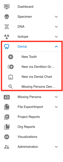
Navigate to the Dental section by opening the navigation bar and selecting the Dental dropdown. For Report Dashboard - please see the Reports documentation.
Create Dental Specimen
Users can create a new dental specimen in multiple ways. For example you can create a single tooth or multiple dental specimens belonging to a dentition bone group such as Maxillary dentition.
New Tooth
User can create a New Tooth by navigate to Left Sidebar Menu -> Dental-> New Tooth. User will be taken to the new dental screen as shown below.
You are now in the create page for the New tooth of the CoRA application. User can create following the below steps.
The screen fields are shown below. Fields in bold are required.
| Attributes | Data Type | Size | Validation Rule | Required/Optional |
|---|---|---|---|---|
| Accession | String | 32 chars | Can only contain letters, numbers, dash and space and should have min 3 chars | Required |
| Provenance1 | String | 32 chars | Can only contain letters, numbers, dash and space | Optional |
| Provenance2 | String | 32 chars | Can only contain letters, numbers, dash and space | Optional |
| Designator | Alphanumeric | 32 chars | Can only contain letters and numbers | Required |
| Tooth | Id | id | valid bones via dropdown | Required |
| Completeness | String | 16 chars | valid completeness via dropdown (Complete, Incomplete) | Required |
New via Dentition Bone Group
To create a multiple specimens via dentition bone group - navigate to the Left Sidebar Menu -> dental -> New via Dentition Bone Group. You will be taken to the new specimens via bone group screen. Here you can create multiple dental specimens that belong to the same dentition bone group.
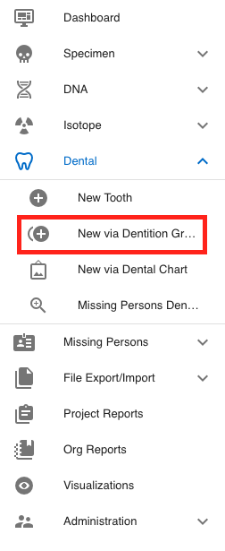
You are now in the create page for the new dental via dentition bne group of the CoRA application. User can create following the below steps.
The fields to create a new bone group are:
- Bone Group
- Grouping
- Bone group
- Side (defaulted to 'Left')
- Completeness (defaulted to 'Complete')
- Accession
- Accession Number
- Provenance 1
- Provenance 2
- Designator
- Pathology
- Traumas
- Pathologies
- Taphonomies
The bolded fields are required.
| Attributes | Data Type | Size | Validation Rule | Required/Optional |
|---|---|---|---|---|
| Bone Group | String | 64 chars | can only contain letters | Required |
| Bone Group Id | String | 64 chars | valid UUID, auto generated | Required |
| Side | String | 8 chars | valid sides via dropdown (Left, Right, Middle, Unsided) | Required |
| Completeness | String | 16 chars | valid completeness via dropdown (Complete, Incomplete) | Required |
| Accession | String | 32 chars | can only contain letters, numbers, dash and space and should have min 3 chars | Required |
| Provenance1 | String | 32 chars | can only contain letters, numbers, dash and space | Optional |
| Provenance2 | String | 32 chars | can only contain letters, numbers, dash and space | Optional |
| Starting Designator | Alphanumeric | 32 chars | can only contain letters and numbers | Required |
New via Dental Chart
To create a new specimens via Dental Chart - navigate to the Left Sidebar Menu -> dental -> New via Dental Chart. You will be taken to the create Teeth by Dental Chart.
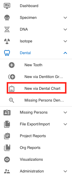
You are now in the create page for the new dental via dental chart of the CoRA application. User can create following the below steps.
The bolded fields are required. The user is required to select Tooth or Dental Code for this report.
The italicized fields are optional if one of the required fields is selected
The fields to create a new bone group are:
- Accession Number
- Provenance1
- Provenance2
- Starting Designator Number
- Bone Group* (defaulted to 'Skull')
- Completeness
- Numbering System* (defaulted to 'Universal')
- Tooth Selection (defaulted to 'Whole Tooth' but we can select from the required options)
-
Dental Code
-
Apply Dental Codes on click: When selected, clicking on a tooth assigns the selected Dental Code to that tooth.
- Clear Dental Codes on click: When selected, clicking on a tooth removes any assigned Dental Code.
Your new dental chart will now be saved, when clicked on save option
if the bone group selected is Mandibular dentition, below dental chart will be presented

if the bone group selected is Maxillary dentition, below dental chart will be presented

Missing Person Dental Comparison Report
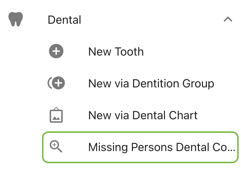
For more information on this report, please go here: Missing Person Dental Comparison Report.
Isotopes and Isotope Batch
Isotope
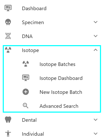
Isotopes can be an important step in the identification process of missing persons. If your project chooses to use Isotope analysis as part of your identification process then you have come to the right place. Here you will learn more about the Isotope modulein CoRA. A critical first step is to cut a sample of the specimen for Isotope analysis and then assign a sample number to it for tracking purposes and after you get results from your Isotope lab you can capture Isotope information here to create an Isotope Profile for further analysis.
Create a Isotope Sample
The Isotope sample and Profile are associated with a specimen, so you must first choose a specimen for which you want to create a Isotope sample for. You can choose a specimen by navigating to the specimen screen from either the specimen search results screen or from any data table row that has a specimen link on it. All search and reports screens have specimen links on them. Simply click these links to navigate to the specimen view/edit screen. Once on the specimen screen you can navigate to the Specimen Action or Details, and then to the Isotope Profile menu.
CoRA's intellisense will automatically take you to the Create Isotope sample screen, if this is the first Isotope sample you are trying to create for this specimen or will take you to the Isotope list screen if a Isotope Sample was previously created for specimen. Note you can create multiple Isotope samples for a specimen.
Tip
CoRA allows you to create multiple Isotope samples for a specimen. If you have multiple isotope samples, CoRA will create a Consensus Isotope Profile for you with data from the multiple samples. Consensus Isotope Profile is a powerful feature of CoRA.
The screen fields are shown below. Fields in bold are required.
| Attributes | Data Type | Size | Validation Rule | Required/Optional |
|---|---|---|---|---|
| Sample Number | Alphanumeric | 8 chars | can only contain letters and numbers | Required |
| Lab | Id | id | valid labs via dropdown setup for the org | Required |
| External Case Number | String | 32 chars | Optional |
Clicking Save will take you to the Isotope Profile screen. You can visit the Isotope Profile screen once you have received data from your Isotope processing lab to enter Isotope related data.
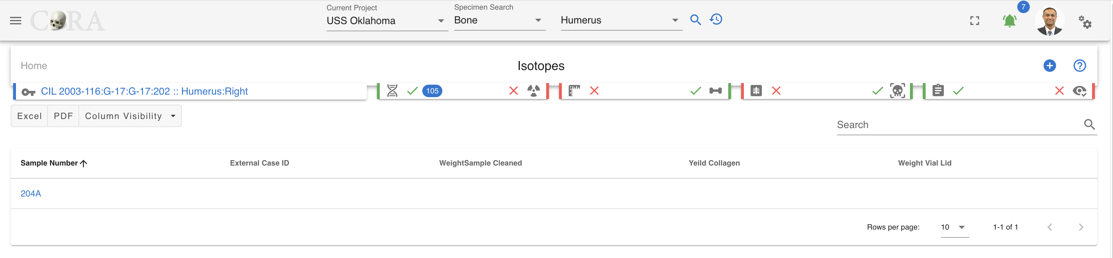
Edit Isotope Profile
Specimens which have had a Isotope sample successfully created will have an associated Isotope Profile. The Isotope profile contains all the relevant Isotope attributes and are editable via action (user must have appropriate role and permissions).
You can visit the Isotope Profile screen once you have received data from your Isotope processing lab to enter Isotope related data to build the Isotope Profile for the specimen. On this screen click the pencil icon on the top right corner to edit the Isotope profile.
The screen fields are shown below. Fields in bold are required.
| Attributes | Data Type | Size | Validation Rule | Required/Optional |
|---|---|---|---|---|
| Sample Number | Alphanumeric | 8 chars | can only contain letters and numbers | Required |
| Lab | Id | id | valid labs via dropdown setup for the org | Required |
| External Case Number | String | 32 chars | Optional | |
| Isotope Batch Number | Number | valid numeric value | Optional | |
| Results Status | String | 32 chars | valid results status via dropdown | Optional |
| Sample Cleaned Weight | Decimal | Optional | ||
| Demineraliing Start Date | Date | Optional | ||
| Demineraliing End Date | Date | Optional | ||
| Sample Vial and Lid Weight | Decimal | Optional | ||
| Weight Collagen | Decimal | Optional | ||
| Yield Collagen | Decimal | Optional | ||
| Collagen Weight used for Analysis | Decimal | Optional | ||
| Analysis Requested | String | Optional | ||
| Well Location | String | Optional | ||
| Carbon Delta | Decimal | Optional | ||
| Carbon Weight | Decimal | Optional | ||
| Carbon Percentage | Decimal | Optional | ||
| Nitrogen Delta | Decimal | Optional | ||
| Nitrogen Weight | Decimal | Optional | ||
| Nitrogen Percentage | Decimal | Optional | ||
| Carbon/Nitrogen Ratio | Decimal | Optional | ||
| Oxygen Delta | Decimal | Optional | ||
| Oxygen Weight | Decimal | Optional | ||
| Oxygen Percentage | Decimal | Optional | ||
| Carbon/Oxygen Ratio | Decimal | Optional | ||
| Sulphur Delta | Decimal | Optional | ||
| Sulphur Weight | Decimal | Optional | ||
| Sulphur Percentage | Decimal | Optional |
Click on Save if any of the fields were updated
Tip
The Isotope profile has attributes to track Carbon, Nitrogen, Oxygen, Sulphur and respective deltas, weight, percentage and relevant ratios for further analysis.
Isotope Batch
A new isotope batch can be created by navigating to Left Sidebar Menu -> Isotope -> New Isotope Batch.
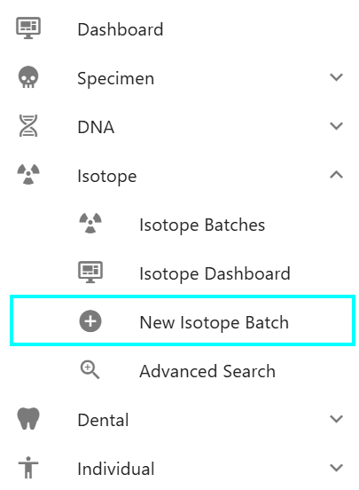
This will allow an Isotope Analyst to first create an isotope batch with a batch number and then associate specimen isotope samples that belong to that batch. After all the isotopes samples are added to the batch we can start processing the isotope batch. The isotope batch will step through multiple processing steps which as detailed below.
We can track the progress throughout the processing cycle of an isotope batch. This functionality will allow the Isotope Analyst digitally document at which step the Isotope Batch is currently in and tracks its' progress and status.
Tip
You must be logged in as an Isotope Analyst in order to create a new isotope batch.

The screen fields are shown below. Fields in bold are required.
| Attributes | Data Type | Size | Validation Rule | Required/Optional |
|---|---|---|---|---|
| Batch Number | Alphanumeric | 8 chars | can only contain letters and numbers | Required |
| Lab | Id | id | valid labs via dropdown setup for the org | Required |
| External Case Number | String | 32 chars | Optional |
Clicking Save will create the isotope batch in the database and will allow you to now associate isotope samples to this batch.
Associate Isotopes Samples
Once an isotope batch has been created the user will be allowed to associate isotope samples to this batch. In order to associate isotope samples to this batch the user must first select the project, this will then show you all the specimen isotope samples that are available to be added to this batch. Selecting the isotope sample and clicking the associate button will move the sample into the associated isotopes list, meaning that the sample has now been added to this batch.
The screen fields are shown below. Fields in bold are required.
| Attributes | Data Type | Size | Validation Rule | Required/Optional |
|---|---|---|---|---|
| Project | Id | id | valid projects via dropdown setup for the org | Required |
| Isotopes Sample | String | 32 chars | Required | |
| Associated Samples | String | 32 chars | Required |
Note
An isotope batch must have at least one isotope sample associated with it.
Start Batch Processing
The start processing button will be enable once isotope samples are associated with the isotope batch. The batch processing has multiple steps and the following sections describe each of these steps in the order they are to be performed. You cannot move forward unless all the tasks in a given step are completed, you can move back to look the data in the previous steps. Only when all steps have been completed can you close out the batch processing. Lets begin by following the steps below.
Note
Each of these steps might take anywhere from a few minutes to multiple hours.
Cleaning
Click the pencil icon on the top right corner to edit the fields in this step.
Each toggle switch must be enabled before moving forwards to the next tab (Demineralizing)
Toggles must be enabled for the following processes:
- Label Tubes and Caps
- Remove all visible signs of surface contamination using rotary tool
- Rinse samples w/dH20
- Sonicate samples with dH20 - cycle 1
- Sonicate samples with dH20 - cycle 2
- Sonicate samples with 95% ethanol
- Sonicate samples with 100% ethanol
- Dry samples in oven
Click Save
After the toggles have been enabled and saved, you will see "Start Date" for Sonicate samples with dH20 - cycle 1, Sonicate samples with 95% ethanol, Dry samples in oven, Sonicate samples with dH20 - cycle 2, Removed cooled samples from tubes, weigh, and return.
Note: Dates cannot be edited, the dates are taken from when the toggle switch was enabled.
After you save the above one new field will appear, enable this toggle once completed and then click save.
- Remove cooled samples from tubes, weigh, and return
Click Save
If you are not able to go to the next tab, please check and ensure all fields and toggles are filled out properly
Demineralizing
Click the pencil icon on the top right corner to edit the fields in this step. Each toggle switch must be enabled before moving forwards to the next tab (Remove Humic Acid).
Toggle must be enabled for:
- Treat samples with 40ml 0.25 M hydrochloric acid until spongy. Change acid every 2-4 days. Treat until there are no hard spots; test with dental pick. Discard waste appropriately.
Click Save
Two new fields will appear, click the pencil icon again to edit to enable the toggle switches.
Toggles must be enabled for:
- Treatment of samples with 40ml 0.25 M hydrochloric acid complete
Note: Dates cannot be edited, the dates are taken from when the toggle switch was enabled.
Click Save
One new field will appear, click the pencil icon again to edit to enable the toggle switch.
Toggles must be enabled for:
- Rinse demineralized samples 3x with dH20
Click Save
You will be moved to the next tab, "Remove Humic Acid", if you are not able to go to the next tab, please check and ensure all fields and toggles are filled out properly
Remove Humic Acid
Click the pencil icon on the top right corner to edit the fields in this step. Each toggle switch must be enabled before moving forwards to the next tab (Solubilizing).
Toggles must be enabled for:
- Treat samples with 40ml 0.125 M sodium hydroxide for 24 hrs. Discard waste appropriately. Rinse samples 5x with dH20.
- Rinse 1 Start
- Rinse 1 End
- Rinse 2 Start
- Rinse 2 End
- Rinse 3 Start
- Rinse 3 End
- Rinse 4 Start
- Rinse 4 End
- Rinse 5 Start
- Rinse 5 End
Click Save
One new field will appear, click the pencil icon again to edit to enable the toggle switches.
Note: Dates cannot be edited, the dates are taken from when the toggle switch was enabled.
- Treatment and Rinse Completed
Click Save
You will be moved to the next tab, "Solubilizing", if you are not able to go to the next tab, please ensure all fields and toggles are filled out properly

Solubilizing
Click the pencil icon on the top right corner to edit the fields in this step. Each toggle switch must be enabled before moving forwards to the next tab (Freeze Drying).
Toggle must be enabled and fields entered for:
- Clean vials and lids. Label.
- Add 15ml pH 3 dH20 to samples and cover tubes with double layer of plastic wrap. Cap tightly.
- Place capped tubes in oven for 24 hours.
- Centrifuge tubes and transfer supernatant into PTFE beakers. Place beakers in oven to evaporate
- Number of Acid-Heat Treatments
- Number of Collagen Transfers
- Close vials and freeze until solid. Tilting vials while freezing can help prevent cracking.
Click Save
You will be moved to the next tab, "Freeze Drying", if you are not able to go to the next tab, please ensure all fields and toggles are filled out properly.

Freeze Drying
Click the pencil icon on the top right corner to edit the fields in this step. Each toggle switch must be enabled before moving forwards to the next tab (Collagen Yield).
Toggles must be enabled for:
- Turn on freeze-dryer. Replace vial lids with Kimwipe caps. Ensure samples are frozen solid.
- Freeze-dry samples - this may take 1 - 3 days. Once collagen is dry, cap vials tightly.
- Freeze-dry samples step completed
Click Save
Note: Dates cannot be edited, the dates are taken from when the toggle switch was enabled.
You will be moved to the next tab, "Collagen Yield", if you are not able to go to the next tab, please ensure all fields and toggles are filled out properly.
Collagen Yield
Click the pencil icon on the top right corner to edit the fields in this step. Each toggle switch must be enabled before the Isotope Batch can be saved.
Toggle must be enabled for:
- Weigh dry samples in vials with lids and record combined weight.
Click Save
You should see "Result Status" field on the top showing that it is Completed.
Isotope Batch Fields
The screen fields are shown below. Fields in bold are required.
Tip
dH2O is Distilled Water
| Attributes | Data Type | Size | Validation Rule | Required/Optional |
|---|---|---|---|---|
| Lab | Id | id | Can choose from the option available | Required |
| External Case # | Alphanumeric | 32 chars | Can only contain letters and numerals | Optional |
| Isotope Batch Number | Alphanumeric | 32 chars | Can only contain letters and numerals | Required |
| Status | String | 32 chars | valid statuses are Open, Associating Isotopes, Cleaning, Demineralizing, Removal Humic Acids, Solubilizing, Freeze Drying Collagen, Determining Collagen Yield and closed | Required |
| Cleaning start date | Date | Required | ||
| Label tubes and caps | Boolean | true/false toggle | Required | |
| Remove all visible signs of surface contamination | Boolean | true/false toggle | Required | |
| Rinse sample with dH2O | Boolean | true/false toggle | Required | |
| Sonicate samples with dH2O-cycle1 | Boolean | true/false toggle | Required | |
| Sonicate samples with dH2O-cycle1 Start Date | Date | Required | ||
| Sonicate samples with dH2O-cycle2 | Boolean | true/false toggle | Required | |
| Sonicate samples with dH2O-cycle2 Start Date | Date | Required | ||
| Sonicate samples with 95% ethanol | Boolean | true/false toggle | Required | |
| Sonicate samples with 95% ethanol Start Date | Date | Required | ||
| Sonicate samples with 100% ethanol | Boolean | true/false toggle | Required | |
| Sonicate samples with 100% ethanol Start Date | Date | Required | ||
| Dry samples start | Boolean | true/false toggle | Required | |
| Dry sample start date | Date | Required | ||
| Dry samples end | Boolean | true/false toggle | Required | |
| Dry sample end date | Date | Required | ||
| Cleaning initials | Alphanumeric | 32 chars | Can only contain letters and numerals | Required |
| Demineralizing Treatment Start | Boolean | true/false toggle | Required | |
| Demineralizing Treatment End | Boolean | true/false toggle | Required | |
| Demineralizing Treatment Start Date | Date | Required | ||
| Demineralizing Treatment End Date | Date | Required | ||
| Rinse Demineralized Samples | Boolean | true/false toggle | Required | |
| Removal Humic Acids treatment start | Boolean | true/false toggle | Required | |
| Removal Humic Acids treatment End | Boolean | true/false toggle | Required | |
| Removal Humic Acids treatment start Date | Date | Required | ||
| Removal Humic Acids treatment End Date | Date | Required | ||
| Removal Humic Acids treatment rinse 1 start | Boolean | true/false toggle | Required | |
| Removal Humic Acids treatment rinse 1 End | Boolean | true/false toggle | Required | |
| Removal Humic Acids treatment rinse 1 start Date | Date | Required | ||
| Removal Humic Acids treatment rinse 1 End Date | Date | Required | ||
| Removal Humic Acids treatment rinse 2 start | Boolean | true/false toggle | Required | |
| Removal Humic Acids treatment rinse 2 End | Boolean | true/false toggle | Required | |
| Removal Humic Acids treatment rinse 2 start Date | Date | Required | ||
| Removal Humic Acids treatment rinse 2 End Date | Date | Required | ||
| Removal Humic Acids treatment rinse 3 start | Boolean | true/false toggle | Required | |
| Removal Humic Acids treatment rinse 3 End | Boolean | true/false toggle | Required | |
| Removal Humic Acids treatment rinse 3 start Date | Date | Required | ||
| Removal Humic Acids treatment rinse 3 End Date | Date | Required | ||
| Removal Humic Acids treatment rinse 4 start | Boolean | true/false toggle | Required | |
| Removal Humic Acids treatment rinse 4 End | Boolean | true/false toggle | Required | |
| Removal Humic Acids treatment rinse 4 start Date | Date | Required | ||
| Removal Humic Acids treatment rinse 4 End Date | Date | Required | ||
| Removal Humic Acids treatment rinse 5 start | Boolean | true/false toggle | Required | |
| Removal Humic Acids treatment rinse 5 End | Boolean | true/false toggle | Required | |
| Removal Humic Acids treatment rinse 5 start Date | Date | Required | ||
| Removal Humic Acids treatment rinse 5 End Date | Date | Required | ||
| Solubilizing clean vials and lids | Boolean | true/false toggle | Required | |
| Solubilizing clean vials and lids date | Date | Required | ||
| Solubilizing add soluble | Boolean | true/false toggle | Required | |
| Solubilizing place in oven | Boolean | true/false toggle | Required | |
| Solubilizing centrifuge tubes | Boolean | true/false toggle | Required | |
| Solubilizing num acid heat treatment | Number | 32 chars | numeric | Required |
| Solubilizing num collagen transfers | Number | 32 chars | numeric | Required |
| Solubilizing freeze vials | Boolean | true/false toggle | Required | |
| Solubilizing freeze vials date | Date | Required | ||
| Freeze Drying Collagen on | Boolean | true/false toggle | Required | |
| Freeze Drying Collagen Start | Boolean | true/false toggle | Required | |
| Freeze Drying Collagen End | Boolean | true/false toggle | Required | |
| Freeze Drying Collagen Start Date | Date | Required | ||
| Freeze Drying Collagen End Date | Date | must be greater than start date | Required | |
| Combined Sample Weight | Boolean | true/false toggle | Optional | |
| Notes | String | 256 chars | Can contains a string alphanumeric values | Optional |
Isotope Dashboard
For more information see the: Isotope Dashboard User Guide.
Individuals
Individuals
An individual is a collection of specimens that the forensic anthropologist believes should go together and belong to an unknown individual. The selection of specimens that go together is done in a blind manner to avoid introducing bias towards the segregation process.
Overview
The Individuals module manages the association of skeletal specimens to unknown individuals. Each individual represents a unique unknown person, and specimens can be grouped together to indicate they likely belong to the same individual based on forensic analysis.
Key Concepts
- Individual Number - Unique identifier assigned to each individual (e.g., I001, I002, I003)
- Specimens - Skeletal elements that are grouped under an individual
- Blind Assignment - The process of assigning specimens without bias
- Individual Profile - Aggregate information (age, sex, ancestry, height) computed from assigned specimens
Accessing Individuals
Navigate to the Individual section from the main menu. This opens the Individuals Management interface where you can view all individuals in the project and perform various operations.
Individual Management
View All Individuals
The Individual Management page displays a list of all individuals in your project with key information:
- Individual Number - Unique identifier for the individual (e.g., CIL 2003-116-G-02)
- Specimens Count - Total number of skeletal elements assigned to this individual
- DNA Count - Number of DNA analysis records associated with the individual
- Identification Date - Date when the individual was identified or case was resolved
- Remains Status - Current status of remains (In Lab or Released)
- Remains Release Date - Date when remains were released if applicable
- Mito Sequence Number - Mitochondrial DNA sequence identifier
- YStr Sequence Subgroup - Displays the Sequence Subgroup
- AuStr Sequence Number - Autosomal Short Tandem Repeat sequence identifier
- Comp Min Age - Estimated minimum age in years
- Comp Max Age - Estimated maximum age in years
- Comp Min Height - Estimated minimum height
- Comp Max Height - Estimated maximum height
- Comp Sex - Display the sex of the individual (if known)
- Comp Ancestry - Ancestry assessment (if known)
Additional Features:
- Search - Use the search field to filter individuals by Individual Number, Identification Date,Remains Status, Mito Sequence Number, YStr Sequence Subgroup, or AuStr Sequence Number
- Column Visibility - Click the Column Visibility dropdown to show/hide columns
- Export - Export the table data to Excel or PDF format
- Refresh - Click the refresh icon to reload the table with current data
- Sort - Click columns header to sort ascending or descending
- Row Actions - Click on an individual row to view details, edit, or delete
Search Individuals
Use the search functionality to quickly find individuals by:
- Individual Number - Search by ID (e.g., I001)
- Notes - Search by notes or comments
- Filters - Filter by status, sex, ancestry, or other attributes
Search Results
The search results display matching individuals with their basic information. Click on any result to view detailed information or edit the record.
DNA Sequence Number Links
In the Individual Management table, the following sequence number columns are clickable and redirect to their respective DNA report pages:
| Column | Description | Redirects To |
|---|---|---|
| Mito Sequence Number | Mitochondrial DNA sequence identifier | Mito DNA Report for the selected individual |
| YStr Sequence Number | Y-Chromosome Short Tandem Repeat sequence identifier | YStr DNA Report for the selected individual |
| AuStr Sequence Number | Autosomal Short Tandem Repeat sequence identifier | AuStr DNA Report for the selected individual |
How to Use
- Navigate to the Individual Management table
- Locate the Mito Sequence Number, YStr Sequence Number, or AuStr Sequence Number column
- Click on any sequence number value in the column
- The page will redirect to the corresponding DNA report for that individual
Example
If an individual has a Mito, Ystr or AuStr Sequence Number of 63-4, clicking on 63-4 will open the Mito DNA Report page showing all mitochondrial DNA analysis results for that individual.
Create Individuals
Manual Creation
To create a new individual:
- Click the plus button in the Individual Management interface
- The Create New Individual form will appear with the following fields:
- Individual Number (required) - Unique identifier for the individual
- Identification Date - Date when the individual was identified or case was resolved
- Remains Status - Current status of remains (dropdown: In Lab / Released)
- Remains Release Date - Date when remains were released if applicable
- Fill in the required Individual Number field
- Optionally enter the identification date, remains status, and release date
- Click SAVE to create the individual, or click CANCEL to discard changes
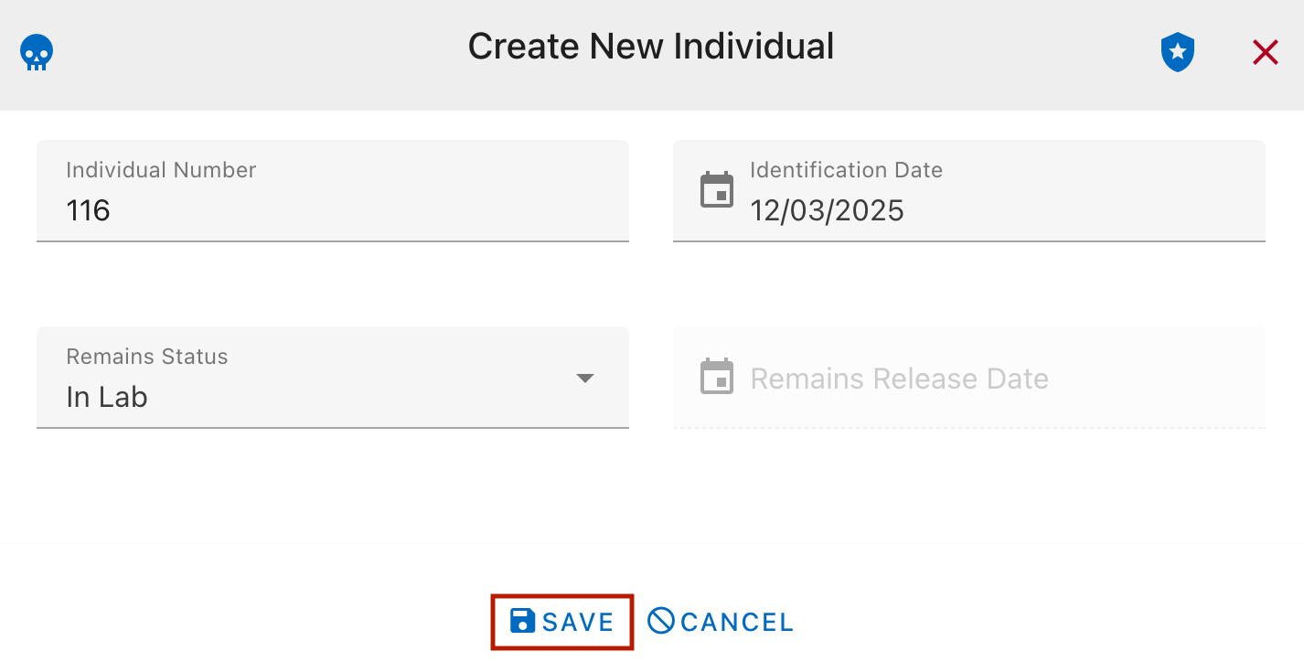
After creating the individual, you can add additional information by editing the record: - Notes - Any observations or comments - Minimum Age - Estimated minimum age in years - Maximum Age - Estimated maximum age in years - Sex - Biological sex determination (if known) - Ancestry - Ancestry assessment (if known) - Minimum Height - Estimated minimum height - Maximum Height - Estimated maximum height
Individual Analytics
The Individual Analytics page serves as a centralized dashboard within the CoRA platform. It is designed to aggregate biological profile data and processing status for specific individuals, allowing researchers to visualize skeletal completion and forensic estimations at a glance.
1. Global Navigation & Context
This section ensures the user knows exactly which set of remains they are analyzing.
- Individual Selection: A primary dropdown menu to select the unique identifier (e.g.,
2003-116-G-02). - Project Context: Displays the current project (e.g.,
USS Oklahoma) and specimen category (e.g.,Bone). - Processing Status: Provides a real-time status tag (e.g.,
"In Lab") and a timestamp of the last data update. - Breadcrumbs: Path tracking:
Home / Individuals
2. Forensic Analysis Tabs
The core of the page is divided into four main biological profile categories. Each tab displays specific methodology and results:
- Age: Methods for estimating chronological age at death.
- Sex: Indicators and methods used for biological sex determination.
- Ancestry: Estimations of biogeographic origin.
- Stature: Mathematical estimations of living height based on long bone measurements.
The Stature Calculation Engine
When the Stature tab is active (as seen in the recording), the system displays a detailed estimation table. It uses specific osteometric data to calculate height:
| Field | Description |
|---|---|
| Specimen Filter | Allows users to focus on specific bones (e.g., Tibia-Left) |
| Method | The specific forensic standard applied (e.g., Trotter and Gleser 1952-WM) |
| Equation | The raw mathematical formula used for the calculation |
| Results | Dynamic output showing Min, Max, and Average height (typically in inches/cm) |
User Guide: Navigating Individual Analytics
Step 1: Select an Individual
To begin your analysis, you must first load the data for a specific set of remains.
- Click the Individual Numbers dropdown menu in the top-left corner.
- Search for or scroll to the desired ID (e.g.,
2003-116-G-02). - The page will automatically populate with that individual's biological data and processing charts.
Step 2: Review the Biological Profile
Once the individual is loaded, navigate through the four core analysis tabs to view forensic estimations:
- Age: View the estimated age range and the methods used to reach that conclusion.
- Sex: Check the determined biological sex and supporting skeletal indicators.
- Ancestry: Review the predicted biogeographic group.
- Stature: Analyze height estimations.
Step 3: Deep Dive into Stature Estimations
The Stature tab is the most data-intensive section. To manage this data:
- Filter Specimens: Use the Specimens dropdown to focus on specific bones (e.g.,
Tibia - Left). - Verify Methodology: Check the Method column to see which forensic standard (e.g.,
Trotter and Gleser) is being applied. - Analyze Equations: Review the Equation column to see the mathematical formula used to generate the height range.
Step 4: Monitor Processing & Completion
Use the interactive pie charts at the bottom to track the lab's progress on the individual:
- Completion Check: Hover over the Complete chart to see the exact ratio of present vs. missing bones.
- Sampling Status: Review the DNA Sampled and Measured charts to ensure all required protocols have been followed.
- Digital Imaging: Check the Scanned, X-ray, and 3D Scanned charts to confirm that a digital twin of the remains has been created.
Step 5: Customize Your Workspace
If the screen feels cluttered, you can tailor the view to your needs:
- Toggle Columns: Click Column Visibility to check or uncheck specific data points (e.g.,
Bone Group,Method Type). - Switch Layouts: Use the List/Grid Toggle (icon with four squares/lines in the top-right) to switch between the dashboard view and a more condensed data list.
- Manual Refresh: If data was recently entered in another module, click the Refresh/Sync icon to update the analytics.
Tip
Always check the Last Updated timestamp and the Status Tag (e.g., In Lab) at the top of the page to ensure you are viewing the most current information.
Individual Analytics Dashboard
Overview
The Individual Analytics page allows users to view, analyze, and visualize biological and computed data for each individual record in the project. It serves as a centralized workspace for both detailed data tables and summary analytics
Each individual may have multiple specimens, and each specimen may have multiple methods for determining:
- Age
- Sex
- Ancestry
- Stature
The page consists of two main sections:
1. Biological Information & Computed Statistic - presented through detailed data table 2. Dashboard Visualization - an interactive set of pie chart widgets summarizing specimen-level data.
Navigation
To access the Individual Analytics, use the left sidebar and select Individual. From the individual menu, choose Individual Analytics The page will appear with various widgets and visual summaries.
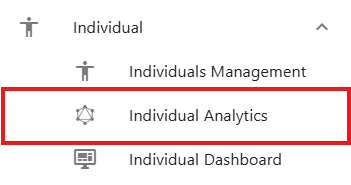
Selecting an Individual
Individual Numbers Dropdown
At the top of the page, users must first select an Individual Number from a dropdown list.

Once selected, the system automatically:
- Loads all associated specimens and methods for that individual
- Retrieves the latest biological and computed statistics
- Refreshes both the data tables and dashboard charts
If any statistics are outdated or missing (for example, computed age or stature), the system automatically updates them before displaying results.
Group option
Next to the dropdown is a Group Checkbox.

When selected, this option groups together all related individual records (for example: CIL 2003-116-G-01, CIL 2003-116-G-01.1, CIL 2003-116-G-01.2) and show all their specimens combined in one view.
This feature is especially useful when multiple individuals are part of a grouped or related case.
Run Stats Button
The Run Stats button allows users to manually refresh computed statistics for the selected individual.

Use this when:
- New specimens have been added or removed.
- Methods have been updated.
- You want to ensure you're viewing the most recent computations without reloading the page.
When clicked, it will:
- Recalculate all relevant stats (age, sex, ancestry, stature).
- Refresh both data tables and dashboard widgets.
Highlight Bar
Located directly below the selection controls, the Highlight Bar summarizes key individual data at a glance.

It includes:
- Total number of specimens
- Identification date
- Remains status
- Remains released date
-
Computed and anthropological (anthro) statistics for:
- Age range
- Stature range
- Sex
- Ancestry
Color coding helps distinguish between computed and anthropological data:
- Computed fields are displayed in green
- Anthro fields are displayed in orange
Each icon in the bar includes a tooltip - hover over it to see what data it represents
Edit an Individual
Clicking an icon in the Highlight Bar opens the Edit Individual form. Within this form, users can update:
- Identification Date
- Remains Status
- Remain Release Date
-
All anthropological statistics, including:
- Minimum Age & Maximum Age
- Minimum Height & Maximum Height
- Sex
- Ancestry
To exit the form, users can either click the Cancel button or click an icon in the Highlight Bar again.
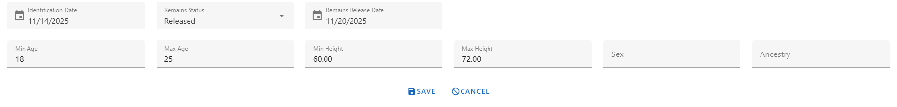
Biological Information Data Table
This section displays all biological and computed data for selected individual. It is organized into four data tabs, each corresponding to a key biological dimension:
- Age
- Sex
- Ancestry
- Stature
Each tab contains a data table with a consistent structure, allowing users to customize visible columns.
Common Table Features
Each table shares the following structure and controls
| Column Name | Description |
|---|---|
| Specimen Key | Unique identifier for the specimen |
| Bone / Bone Side / BoneGroup | Anatomical references for each specimen |
| Method Name / Type / Feature | Details about the method used to compute the stat. |
| Computed Statistic | Displays calculated results depending on the tab (age range, sex, ancestry, or stature values). |
| Individual Number | (Optional) Can be show or hidden via the Column Visibility menu. |
| Created At / Updated At | (Optional) Metadata columns for record history. |
Users can toggle optional columns through the Column Visibility Dropdown, located at the top left of each table.
A Last Updated Timestamp is displayed next to the Column Visibility menu, showing when the individual's data was last refreshed.

Collapse & Expand Table
Users can collapse or expand the data table by clicking the Collapse/Expand button located next to the Column Visibility menu.
- Collapse reduces the table to its header area, giving users more space to focus on other page components or customize their layout.
- Expand restores the table to full view when users need to review or interact with its data again.
This helps users tailor the workspace to their personal viewing preferences.
Age Tab
This tab displays the computed Minimum and Maximum Age values for each specimen and methods. Each row represents a method used on a specimen, showing the resulting age range derived from the method's parameters. Use this tab to compare multiple age estimation methods and verify consistency across specimens.
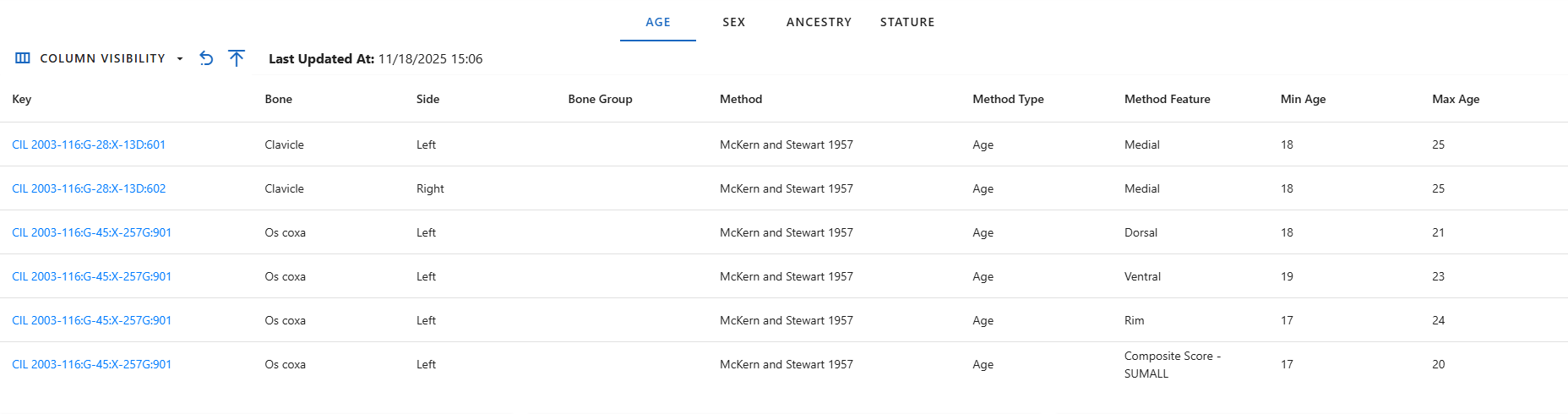
Sex Tab
The Sex tab lists all methods used to estimate biological sex and their computed outcomes. Each row displays the specimen and bone analyzed, the method used for determination, and the Computed Sex result. This view helps users quickly assess which specimens have reliable sex determinations and which require further review.
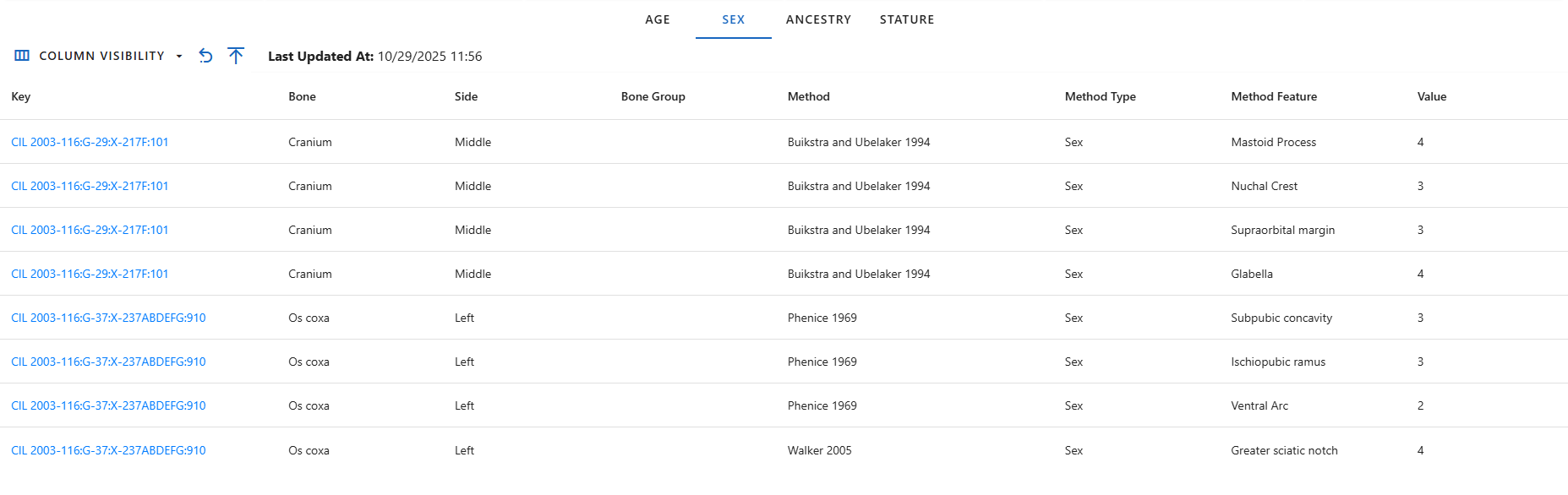
Ancestry Tab
This tab shows computed Ancestry results for each specimen and method applied. The ancestry values are derived from various metric and non-metric analyses and can be compared across multiple methods. This helps identify consistency in ancestry determinations and validate the underlying analytical methods.
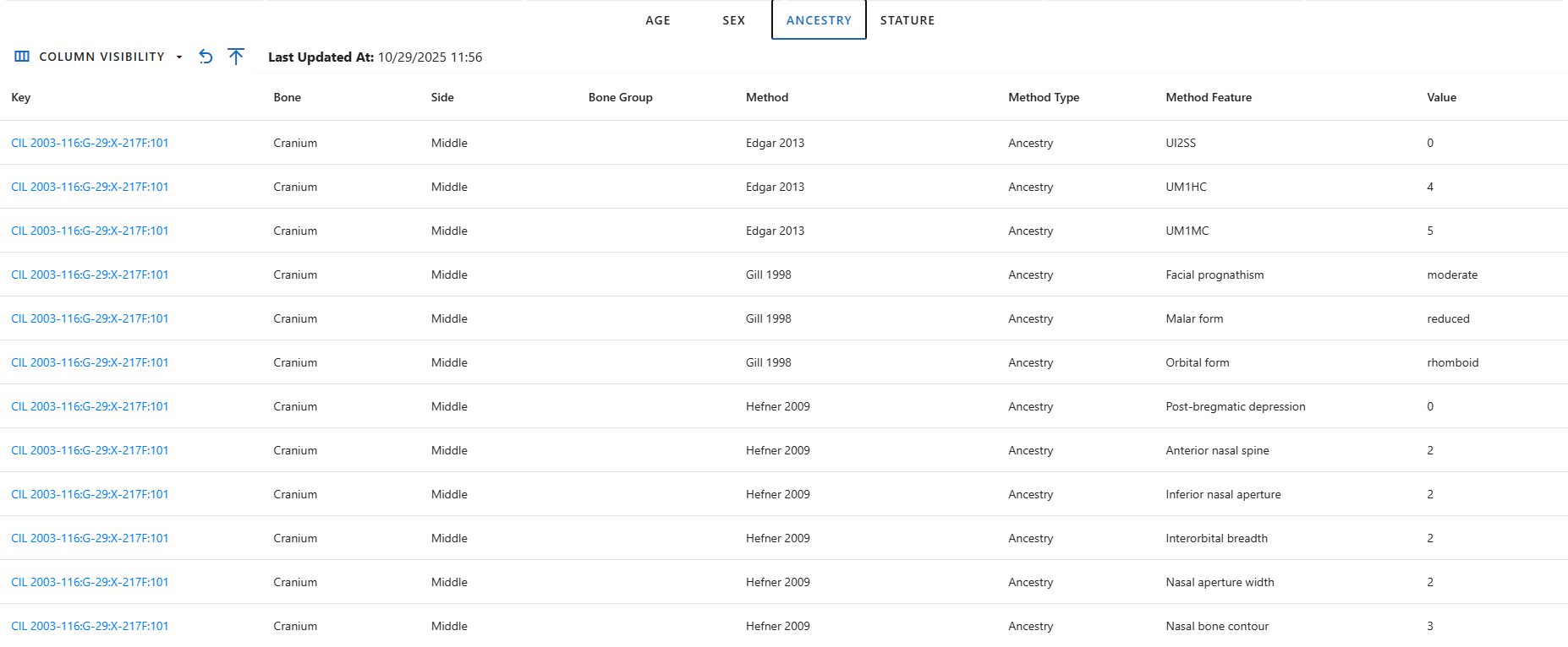
Stature Tab
The Stature tab is the most detailed, as it contains multiple calculated values per specimen and selected method. It includes minimum, maximum, and average computed height, equation used, and the bone measurement. The absolute minimum and maximum height across all specimens are highlighted in blue, allowing users to quickly identify overall stature range boundaries.
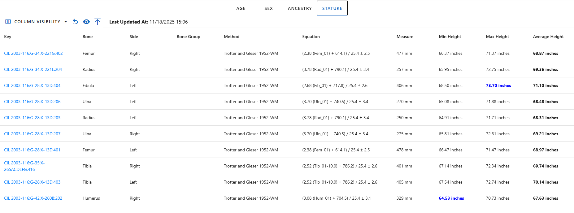
When on the Stature tab, three additional dropdown menus appear above the table:
- Specimens Dropdown - Show list of specimens that was used to calculate stature.
- Methods Dropdown - Choose which calculation method to display. Each project has a predefined default method.
- Unit Dropdown - Choose display units for height (default: inches).

Beside these dropdowns, the Go to Visualization button appear on the right of the Column Visibility menu, which redirects users to the Stature Estimation Visualization page. All selected filters (individual, specimen, method , and unit) are passed to the visualization page automatically.

Analytics Dashboard
The lower section of the page presents the Individual Dashboard, a visual summary of specimen-related data using pie charts. These charts provide immediate insight into the completeness, sampling, and analytical coverage of all specimens for the selected individual.
Widget Controls & Interactive Features
The dashboard provides several interactive features that allow users to customize and explore the displayed data widgets according to their preferences. These interactions help users focus on specific insights and personalize their dashboard layout.
Rearranging and Removing Widgets
Users can rearrange all widgets on the dashboard by dragging and dropping them to new positions. Additionally, users can remove widgets they do not wish to view. All layout changes, including widget positions and removals, are automatically saved in the browser cache, ensuring that when users return to the dashboard later, their customized layout is preserved.
Collapse and Expand Widgets
Each widget includes an option to collapse or expand its view.
- Collapsed View: Minimized the widget to show only its header, helping reduce clutter.
- Expanded View: Restores the full widget for complete data visibility.
In addition to per-widget controls, the dashboard provides global Collapse All and Expand All buttons located at the top-left of the screen, just below the Profile and Settings section. These controls allow user to quickly minimize or restore all widgets simultaneously, making it easier to manage the dashboard's overall layout and focus on specific areas of interest.
Hover for Details
When users hover over chart elements, additional details appear in a tooltip. This feature provides deeper insight into specific data points without cluttering the main visualization.
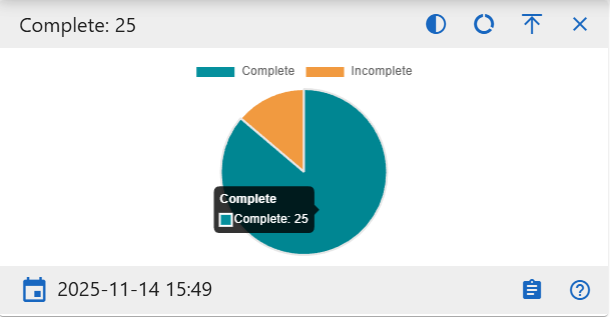
Chart View Customization
Several widgets support changing the chart style to fit user preference or data interpretation needs:
- Full Circle and Semi-Circle Toggle: Users can switch between a full circular chart view and a semi-circular (half-donut) view for a more compact display
- Pie and Donut Toggle: Users can switch between pie and donut chart styles to adjust visualization clarity and style.
Data Freshness
Each widget displays a Last Updated Timestamp to confirm when the data was last refreshed.

Detail Views
Each widget includes a Details button that opens a detailed table view.

The Detail Page provides:
- A complete record list for the selected chart category
- Table search and filter capabilities
- Export options (Excel and PDF)
- Column Visibility controls
This allows users to explore specific specimen-level data in depth while maintaining consistency with other dashboards.
Widget Details
Below are description of each dashboard widget and what it represents. All charts are showing the specimen data for the selected individual.
Complete
Show the proportions of specimens marked as Complete vs. Incomplete. Useful for quickly assessing case completion status.
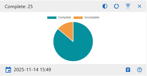
DNA Sampled
Displays how many specimens have DNA samples collected. Use this to identify which specimens still need sampling.
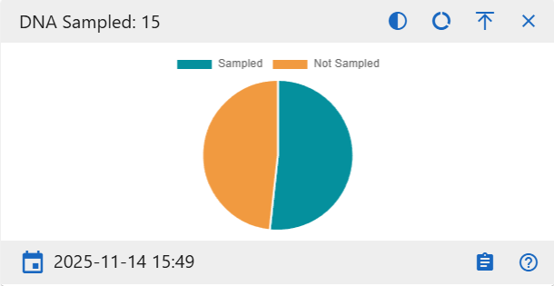
Measured
Visualizes how many specimens have measurement data recorded.
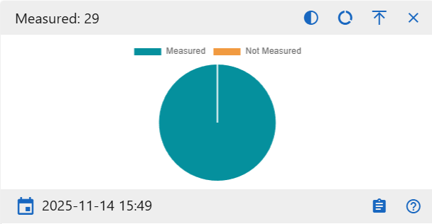
CT Scanned
Show the number of specimens that have undergone CT scanning versus those not scanned.
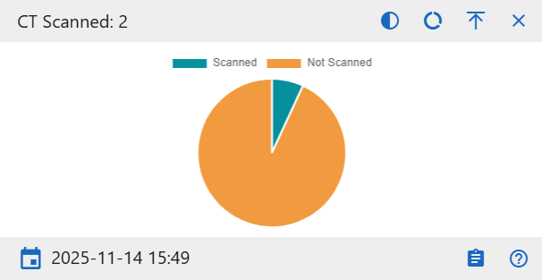
X-ray Scanned
Show the number of specimens that have been X-ray scanned versus those not scanned.
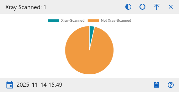
3D Scanned
Display how many specimens include 3D digital scans. This helps monitor digitization completeness for each individual.
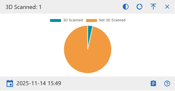
Isotope Sampled
Show how many specimens have isotope data collected for geochemical analysis.
Method Sex
Displays how many specimens that have sex determination methods.
Method Age
Displays how many specimens that have age determination methods.
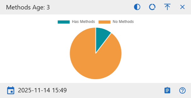
Method Ancestry
Displays how many specimens that have ancestry determination methods.
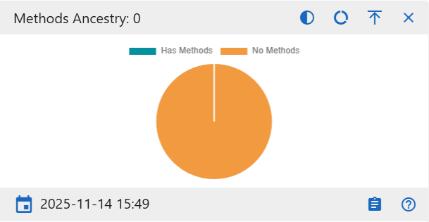
Individual Analytics Dashboard Drilldowns
Overview
A drilldown page provides an in-depth view of a specific chart from the Individual Analytics dashboard. While the dashboard gives a quick, high-level snapshot, the drilldown view presents a larger version of the chart along with a complete table of all specimens represented. This allows you to move from a visual summary to the underlying data behind each part of the chart.
Navigation
You can open drilldown page by selecting the Detail button inside any pie chart widget on the dashboard. Clicking this button loads the dedicated drilldown view for that chart, where you can continue exploring the data with more space and context.
Page Layout and Features
Each drilldown page begins with a full-size versions of the chart you selected. It behaves the same way as the dashboard version, hovering will reveal tooltips, and you can switch between pie and donut views or toggle between full and semi-circle layouts.
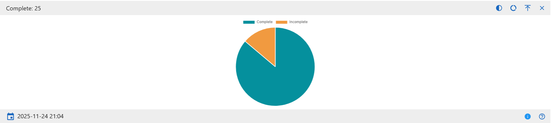
Below the chart is a comprehensive data table showing all specimens included in the visualizations. The table supports sorting, searching, and hiding or showing additional columns, allowing you to explore the dataset from multiple angles.
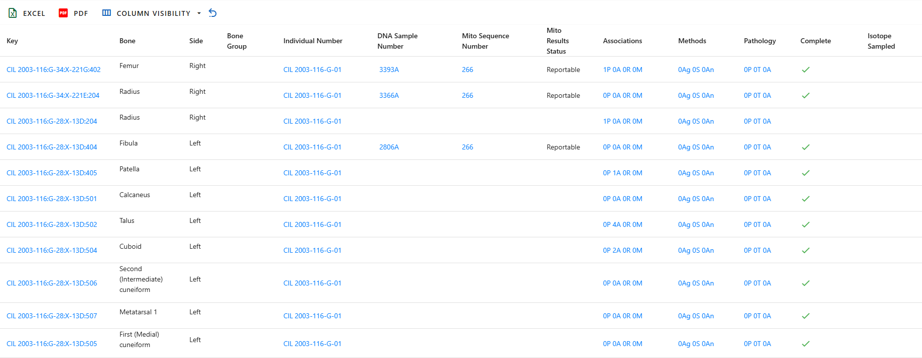
Data Table Columns
The drilldown page includes a comprehensive specimen data table. Each row represents a single specimen, and each column provides a specific attribute, measurement, administrative detail, or analytic result. Below is a complete explanation of every column available in the table.
- Key - The unique identifier for the specimen, combining accession and provenance information into a single readable label.
- Accession Number - The collection or case accession number assigned by the project or institution.
- Provenance1 - Primary provenience descriptor
- Provenance2 - Secondary provenience descriptor that provides more specific context
- Designator - The additional identifier used internally to label the specimen, often representing sub-designations.
- External ID - An ID assigned by an outside agency or laboratory, if applicable
- Bone - The specific bone (e.g, Femur, Humerus)
- Side - Indicates whether the specimen is from the left side, right side, or is midline
- Bone Group - A broader grouping of bones, used for sorting and filtering
- Individual Number - The assigned number for the biological individual this specimen belongs to
- Identification Date- The date the individual was identified
- Remains Status - The current status of the remains (e.g, In Lab, Released)
- Remains Release Date - The date the remains was released, if applicable
- DNA Sample Number - Identifier fpr the DNA sample taken from the specimen
- Mito Sequence Number - The mitochondrial DNA sequence ID assigned during analysis
- Mito Results Status - Indicates the confidence or success level of the mitochondrial sequencing results
- Associations - Summarizes how many associations the specimen has across four categories: Articulations, Pair Matches, Refits, and Morphology
- Methods - Shows the number of analytical methods applied to the specimen across these three categories: Age, Sex, and Ancestry
- Pathology - Displays howmany recorded findings the specimen has across three pathology related categories: Pathology, Trauma, and Anomaly
- Taphonomy - Information about environmental or postmortem processes affecting the specimen
- Tags - Any special flags or metadata attached to the specimen
- Dental Codes - Dental notation or coding related to definition
- Measured - Indicates whether measurements have been taken for the specimen
- Complete - States Whether the specimen is complete or incomplete
- Isotope Sampled - Indicates whether an isotope sample was taken
- Clavicle Triage - Status of clavicle triage evaluation
- Count - Quantity count when multiple pieces are associated with the same item
- Mass - The mass or weight of the specimen, if recorded
- Min Age - The computed minimum age for the specimen
- Max Age - The computed maximum age
- Custom Field ½/3 - Additional values defined by the project for specialized use
- CT Scanned - Whether CT scanning was completed for the specimen
- CT Scanned At - The date of the CT scan
- Xray Scanned - Whether X-ray imaging was performed
- Xray Scanned At - The date of the X-ray scan
- 3D Scanned - Whether 3D scanning was performed
- 3D Scanned At - The date of the 3D scan
- Inventoried - Indicates whether an inventory check was complete
- Inventoried By - Name of the person who performed the inventory
- Inventoried At - Date the inventory was complete
- Reviewed - Shows whether a review or secondary check was performed
- Reviewed By - Reviewer's name
- Reviewed At - Date of the review
- Created By - User who first created the record
- Created At - Date the record was originally created
- Updated By - User who most recently modified the record
- Updated At - Date of the latest update
Dashboard Chart Description
Complete
Categories:
- Complete
- Incomplete
This chart shows how many specimens have undergone DNA sampling. The Sampled category counts specimens that have been processed for DNA extraction, while Not Sampled reflects those without any DNA sampling activity
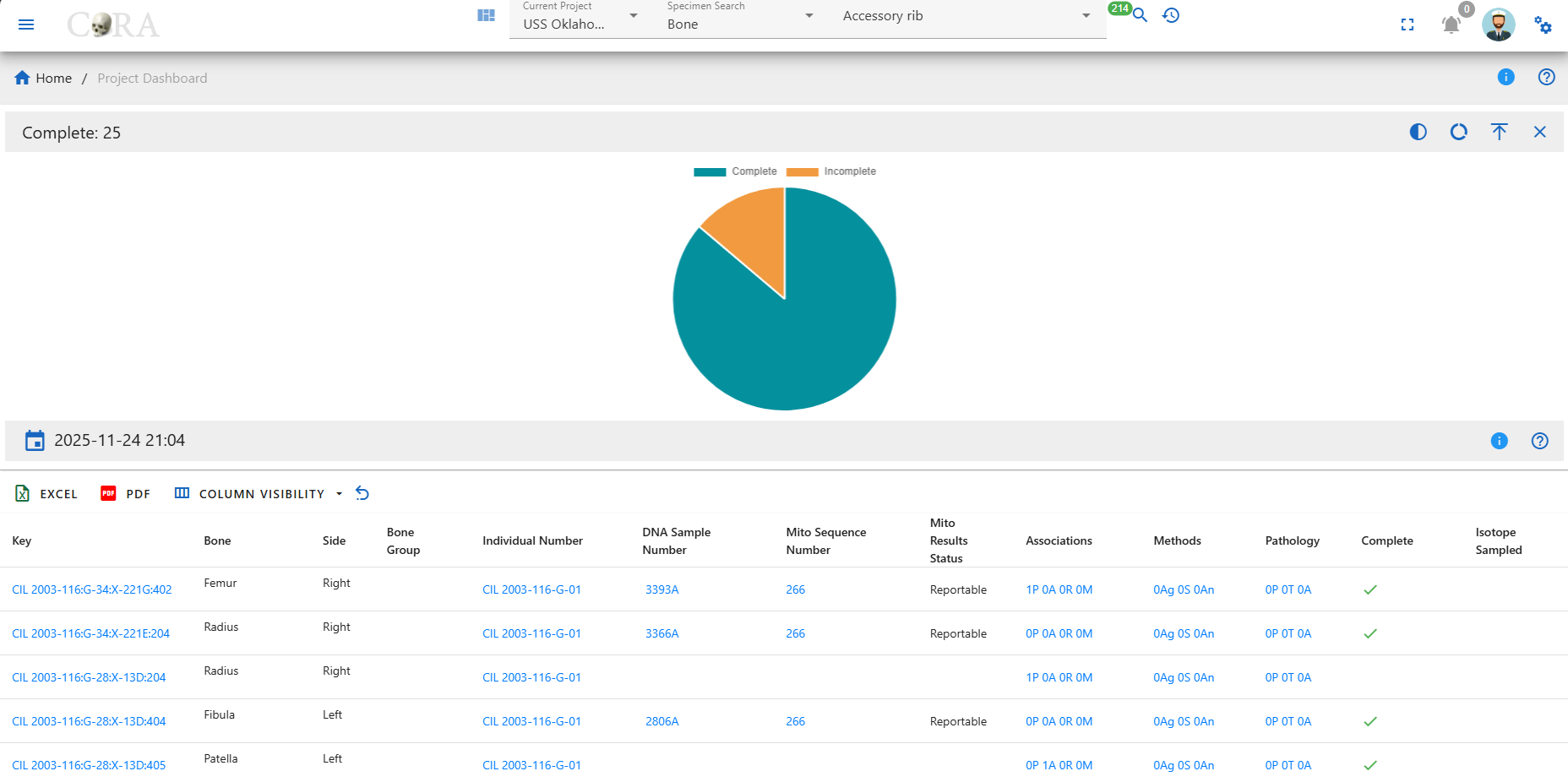
DNA Sampled
Categories:
- Sampled
- Not Sampled
This chart shows how many specimens have undergone DNA sampling. The Sampled category counts specimens that have been processed for DNA extraction, while Not Sampled reflects those without any DNA sampling activity.
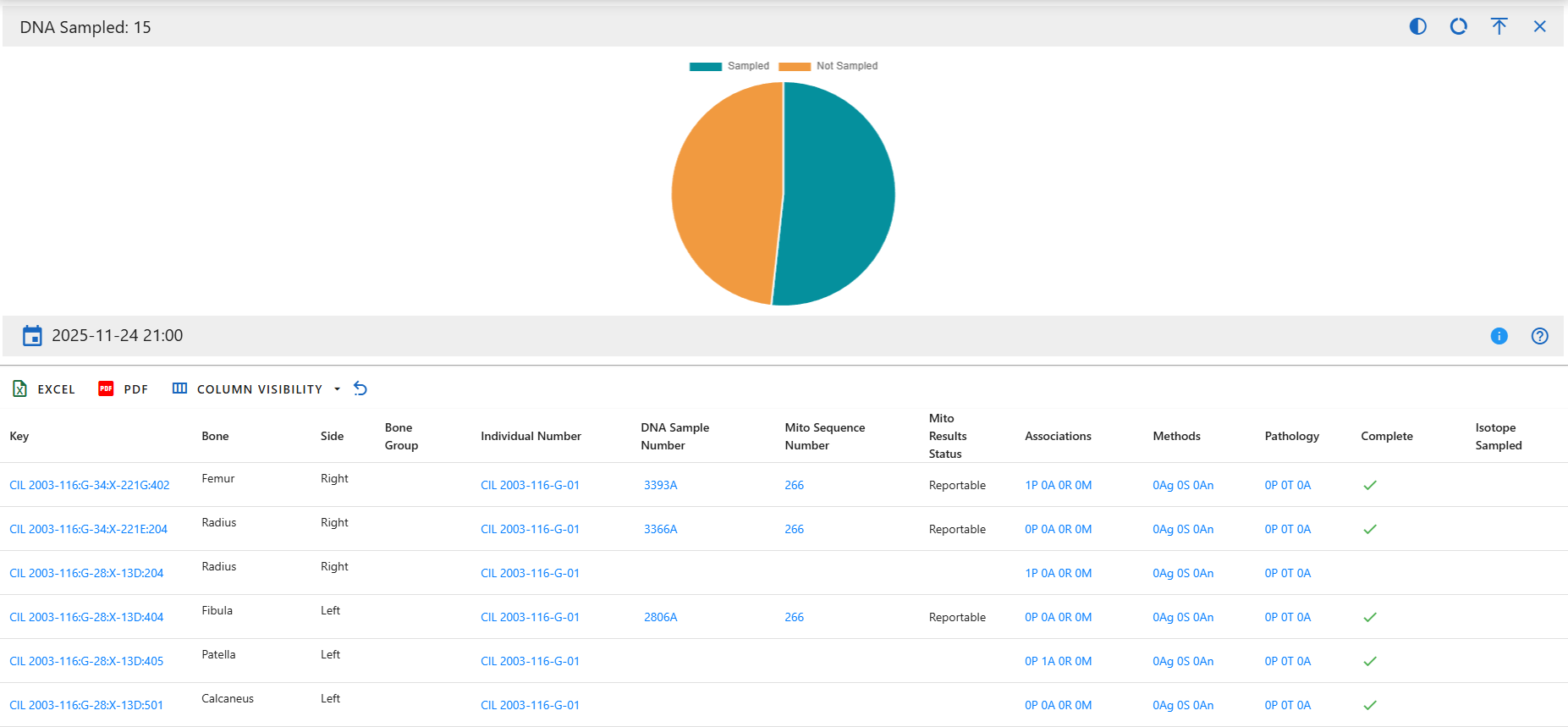
Measured
Categories:
- Measured
- Not Measured
This chart displays whether specimens have recorded osteometric measurements. Measured specimens contain at least one measurement entry, while Not Measured specimens have no measurement data recorded.
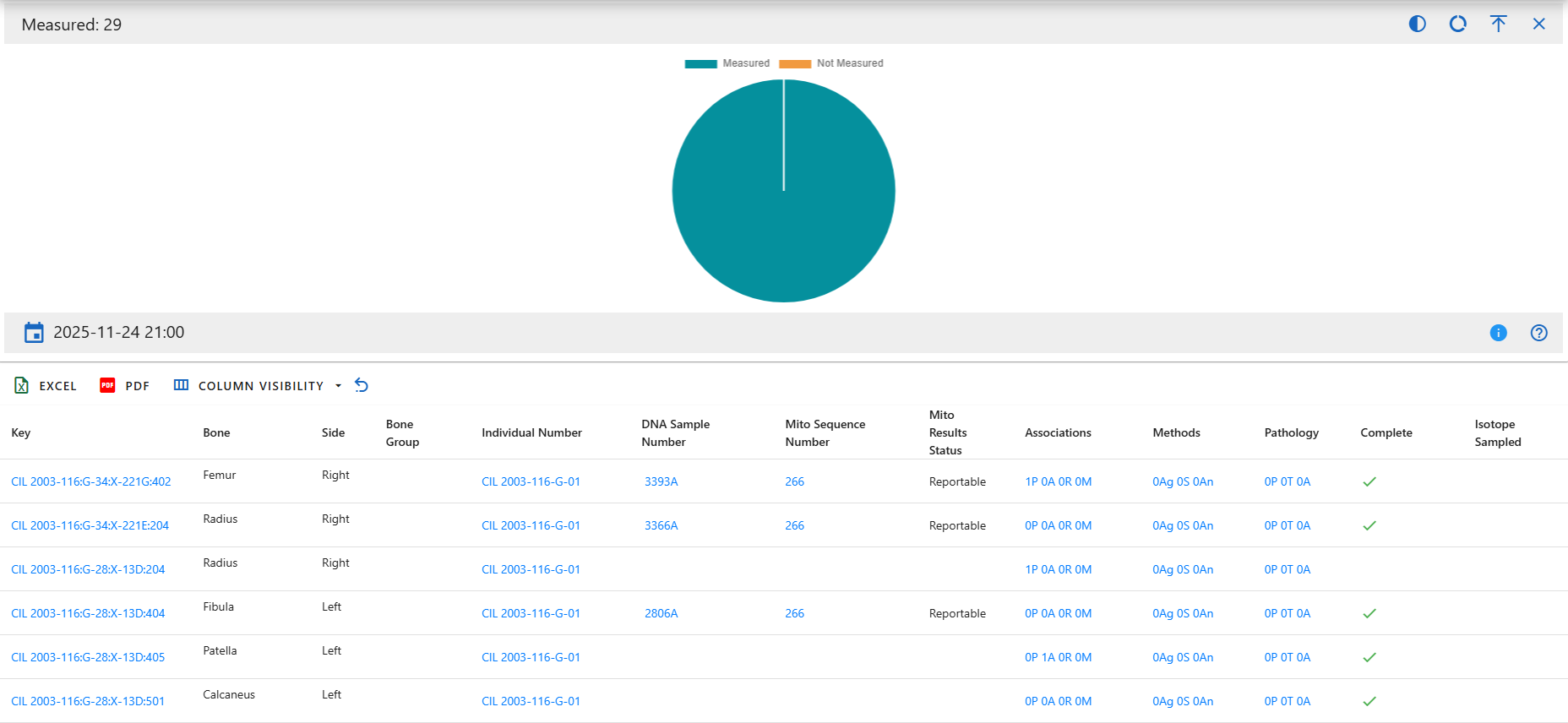
CT Scanned
Categories:
- Scanned
- Not Scanned
This chart indicates which specimens have been scanned using CT technology. Scanned specimens have CT scan data associated with them, while Not Scanned do not.
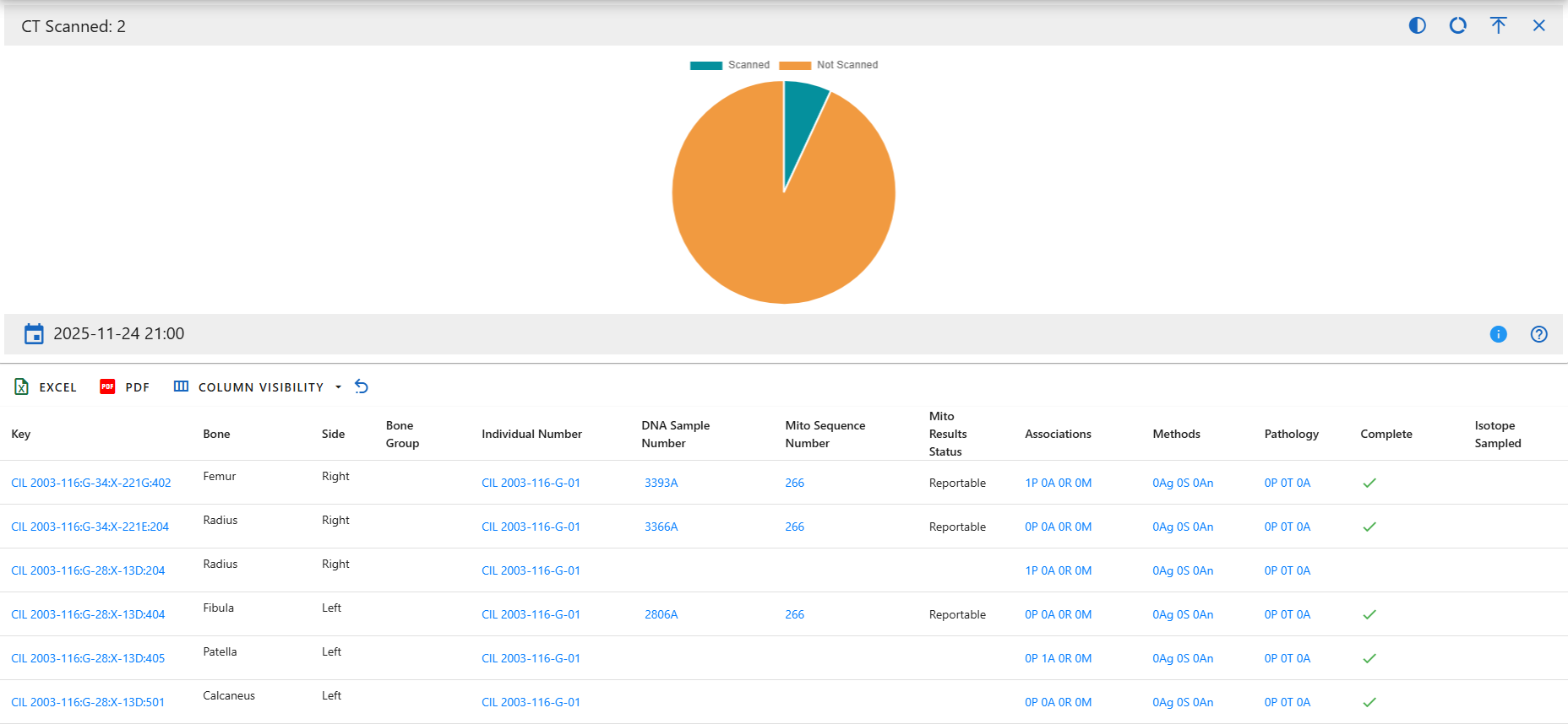
X-ray Scanned
Categories:
- Xray Scanned
- Not Xray Scanned
This chart shows the number of specimens with associated X-ray imaging. Xray Scanned reflects specimens that underwent radiographic imaging, and Not Xray Scanned shows those without X-ray records.
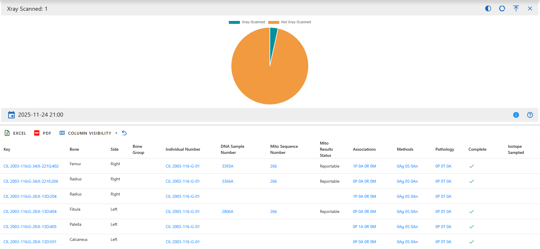
3D Scanned
Categories:
- 3D Scanned
- Not 3D Scanned
This chart displays whether specimens were captured using 3D scanning technologies (e.g., structured light, laser scanning). 3D Scanned indicates digital 3D models exist, while Not 3D Scanned shows specimens lacking such models.
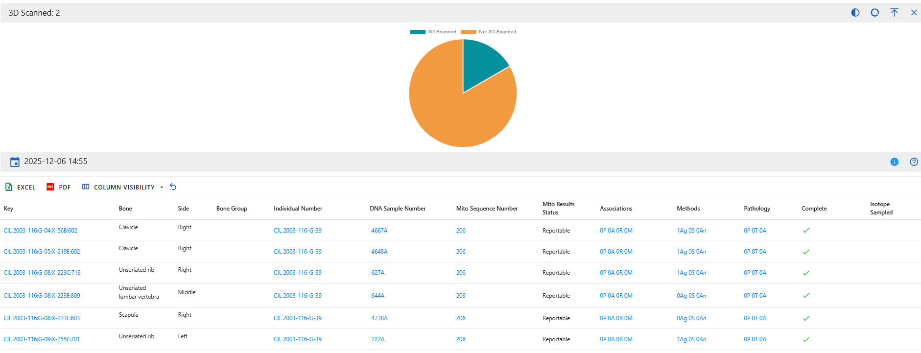
Isotope Sampled
Categories:
- Sampled
- Not Sampled
This chart tracks whether specimens have undergone isotopic sampling (e.g., strontium, carbon, nitrogen analysis). Sampled indicates an isotopic test has been performed, Not Sampled indicates no record of sampling.
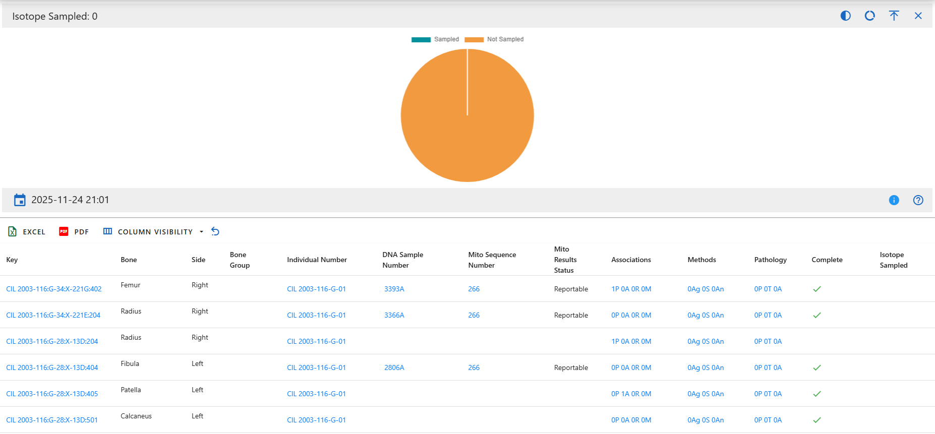
Methods Sex
Categories:
- Has Methods
- No Methods
This chart counts how many specimens have at least one sex estimation method applied. Has Methods includes specimens with sex analysis (e.g., pelvis morphology, cranial features). No Methods indicates no sex-related methods were recorded.
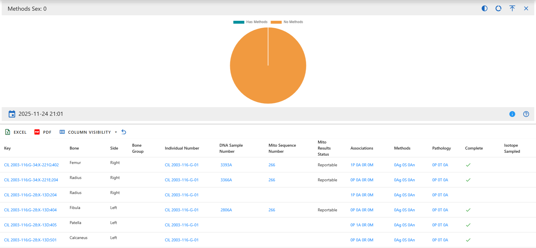
Methods Age
Categories:
- Has Methods
- No Methods
This chart indicates whether age estimation methods have been applied to specimens. Has Methods reflects specimens where age estimation was performed. No Methods shows specimens without age-related analysis.
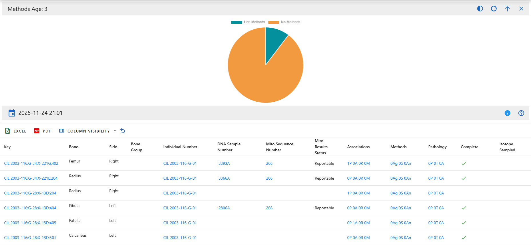
Methods Ancestry
Categories:
- Has Methods
- No Methods
This chart shows whether ancestry estimation methods were applied. Has Methods includes specimens analyzed for ancestry (e.g., metric or morphoscopic traits). No Methods indicates no ancestry analyses were recorded.
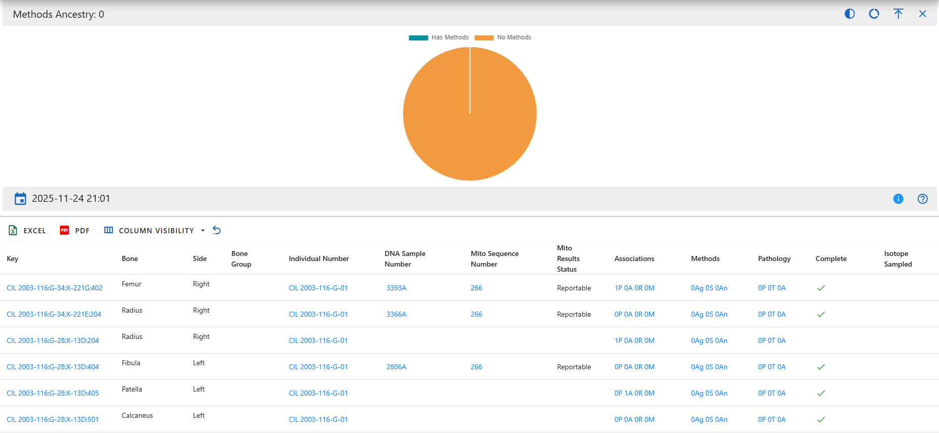
Missing Persons
The missing persons module in CoRA is where you create and manage records of missing persons. In CoRA there are two roles that manage this module. The role of missing persons administrator (mp admin) and missing persons case manager (mp case manager) administer and manage the missing person cases.
Navigation
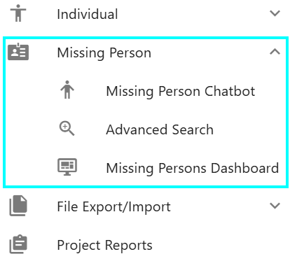
Navigate to the Missing Persons section by opening the navigation bar and selecting the Missing Persons dropdown. From there select Advanced Search to go to the Missing Persons Search page.
For Missing Persons Report Dashboard - please see the Reports documentation.
Searching Cases
Users can search missing persons cases by navigate to Left Sidebar Menu -> Missing Persons-> Advanced Search.

You are now in the advanced search for the Missing Persons section of the CoRA application.
The Missing Persons module of the CoRA application comes with a powerful searching tool, you can use this generate an advanced search of missing persons cases using a wide array of criteria.
Advanced Search
The advanced search allows you to find missing person cases with a variety of different filters. Any filters set will be combined to find records that match all of the criteria.
The fields to search a missing person case are as follows:
- Case Status
- Owner Service - Filters by service that owns the record in DCIPS
- Service Member Service - Filters by the service that the service member belonged to
- Conflict
- Incident - Case insensitive search for any incident containing the value entered.
- DPAA Case Status - Whether the case is marked as resolved or unresolved
- DPAA Priority - Numeric value for any priority.
- Case Number - Finds any records containing the value specified in the DCIPS Case Number field.
- Name - Case insensitive search for any name containing the value specified. Searches first, middle, and last name fields along with the suffix.
- Project - Projects available for filtering are limited to those two which the logged in user is assigned.
- Case Manager - Allows selection of any PCRB administrator or case manager for filtering cases assigned.
- PCRB Priority - Case insensitive search of PCRB Priority for any record containing the value specified.
- Genealogy Status - Filters by status of the genealogy request assigned to the missing persons case.
- Updated At - Users are prompted to specify a start and end date to filter by the updated at date field of the missing persons case record.
- DPAA Prioritized Only - Activating this filter excludes all missing persons cases without a DPAA priority set.
- Followed Up - Whether the record has been followed up on or not
- Updated DCIPS - Whether the record has been updated in DCIPS
When searching for cases, use some or all of the fields to narrow down the results. Filters are used in combination, so specifying multiple filters will limit the results to those records matching all criteria specified.
Note: In order to search for all of the missing persons cases, leave all fields empty.
Once you have inputted your search criteria, select the "Generate" button from the toolbar to search.
![]()
Working with Search results
After generating search results, you can further refine, filter, and sort your results.
Sorting
Sorting the search results is as simple as clicking on the column header. Clicking once will cause the data to be sorted into ascending order based on the column selected. Clicking the same column header again will cause the data to be sorted in descending order. To clear the filter, click the column header a third time.
Sorting by multiple columns is also possible. To do this, select the column header of the first column by which you wish to sort. Then select the second column header. Numbers will appear next to the column headers allowing you to see which columns are being used to sort.
Searching
Instantly search your advanced search results for any keyword with the search bar on the right side of the page. Simply enter the key you wish to search with and the advanced search results will update accordingly.
Searching advanced search results is robust and will match items that are exact or partial to what you have entered into the search bar.
For example, searching advanced search results for "Smit" would bring up any results that contain "Smit", like "Smith", "Smitty", and "Smite".
Column Visibility
The search results will return the following columns if available. Additional columns are available and can be selected from the "Column Visibility" button above the search results.
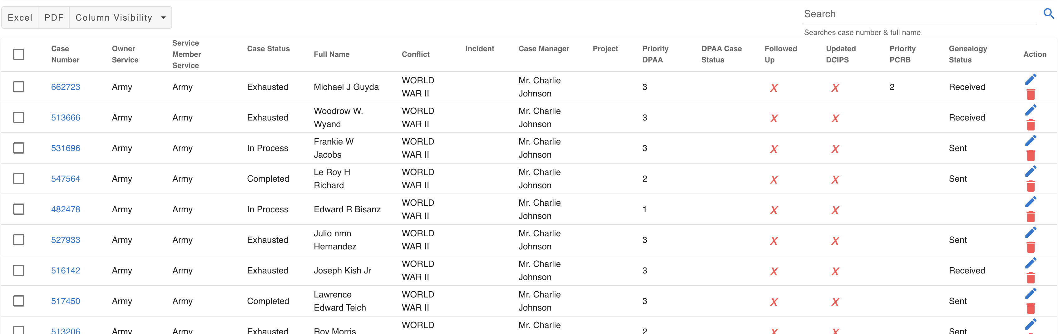
- Case Number
- Case Status
- Owner Service
- Service Member Service
- Full Name
- Conflict
- Incident
- Case Manager
- Project
- Priority DPAA
- DPAA Case Status
- Followed Up
- Updated DCIPS
- Priority PCRB
- Genealogy Status
Download Result Cases
Once you have your advanced search results refined in a way that you like, export this list with the export buttons on the left hand side.
Available export options are:
- Excel
Selecting this option will export the search results in the selected file format for download onto your computer.
Batch Edit
Making changes to many cases at the same time can be performed with the batch editing feature. Once you select multiple cases using the check boxes on the left side of the results of an advanced search an actions menu will appear.
Here you will be able to select "Batch Edit" and update one or more fields for each of the selected cases.
MissingPersonChatbot
Warning
The following section on this page is work in progress.
Managing Cases
CoRA allows you to look at and manage missing person cases with ease and flexibility. Select a specific case by selecting the case number underlined in blue. Once you select the case, a page will open with the details of the selected case.
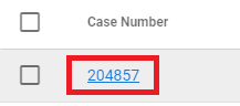
Once you have the case open, interact with the different fields to make the changes you need.
Note: Some of the fields may be grayed out, these are fields that you cannot change and are changed in the system of record or by an individual with more access
Case information is separated into several different categories:
- Basic Case Information
- DPAA
- FRS Status
- Checklist
Basic Case Information
At the top of the page, you will notice the essential information is grouped together:
- DCIPS Case Number
- Owner Service
- Service Member Service
- Service Member Name
- SSN/ASN
- Date of Death (if available)
- DPAA Case Number
- Case Status
- Incident
- Conflict
The card is also outlined in a color to represent the status. These colors correspond with the following statuses:
| Status | Color |
|---|---|
| Completed | Green |
| In Process | Blue |
| Exhausted | Yellow |
| Not Started | No Color |


DPAA
The DPAA section of the case detail page is dedicated to DPAA. The following fields can be found here and modified:
- Project
- DPAA Case Status
- DPAA Priority
- Possible Remains in Lab
- XFile
- Field Grave
- Temp Field Grave
FRS Status
The FRS Status section of the case detail page is dedicated to tracking of Family Reference Samples (FRS). The following fields can be found here and modified:
- 1st mtDNA
- 2nd mtDNA
- 3rd mtDNA
- 1st yDNA
- 2nd yDNA
- 1st nuclear
- 2nd nuclear
Checklist
The Checklist section of the case detail page is dedicated to keeping track of the tasks to perform in reference to the specific case being viewed. The following fields can be found here and modified:
- Add Family members from Genealogy Report to DCIPS
- Attempt contact of family members in DCIPS
- Send Outreach letters to family members unreachable by phone
- Records sent to family
- Followed Up
- Updated DCIPS
This section of the case details also provides the status for the various records relating to the case:
- IDPF Status
- OMPF Status
- CSR Status
- Awards Status
Genealogy Request
The case manager for a case, the missing persons administrator, and the system administrator may generate a genealogy request. Those with permission to generate a genealogy request will see a blue Genealogy Request button to the left of the Save and Cancel buttons.
Clicking on this button will generate and download a pdf titled Request for Genealogy Services.

The pdf will have two sections of information, Service Member Data and Genealogy Search, and three authorization sections with signature and date fields. Even though some of the fields are pre-filled, they are editable.
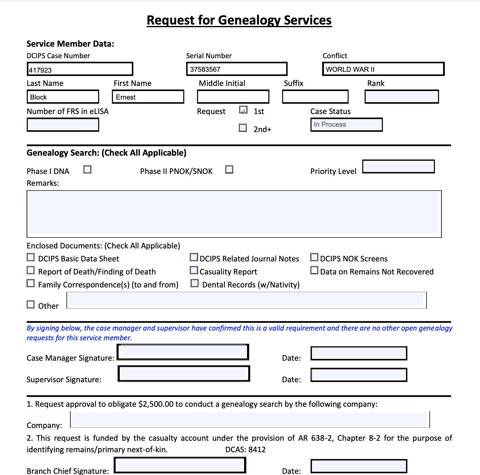
The editable fields on this report are - Rank - Number of FRS in eLISA - Case Status - Priority Level - Remarks - Other field - Case Manager Signature - Supervisor Signature - Company - Branch Chief Signature - Billing Official Signature - GPC Holder Signature - Date fields - All checkboxes
Comments
The Comments section of the case detail page is dedicated to viewing and logging the comments and notes related to the specific case.
To leave a comment, type the comment into the comment text box and click the save icon on the right side.
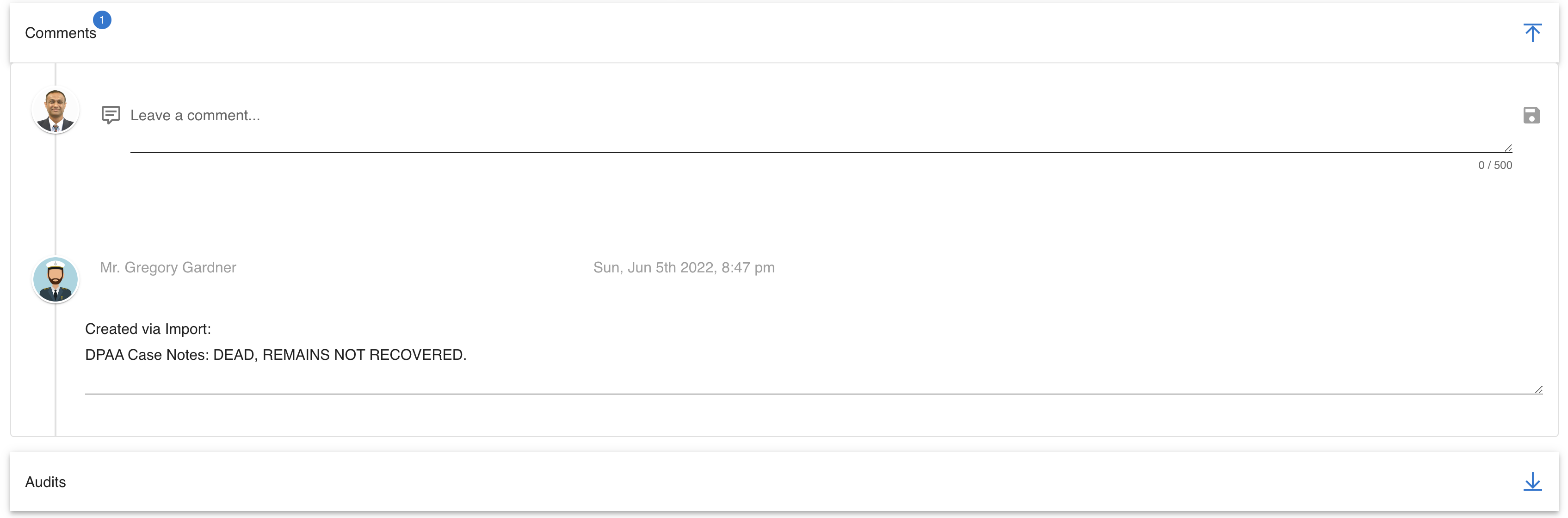
This will save the comment with your username as well as the date and time the comment is made. The comment can be edited or deleted by a system administrator.
Audits
The Audits section allows users to view all changes made to a missing persons record. This will show the detail of what, who, and when changes were made in the system.
To view the audit data, select the arrow on the right side of the Audits section to view any relevant audit records.
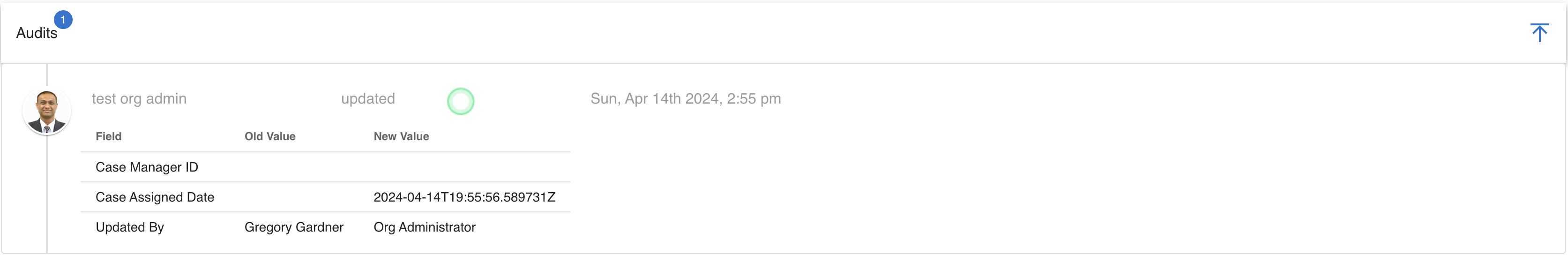
Tags
The tags section enables users to associate additional information (aka Tags) to missing persons records.
Importing Data
Importing case changes and new cases from DCIPS is made easy with CoRA's robust import capability. To start the file import process, navigate to Left Sidebar Menu -> File Export/Import-> File Import.
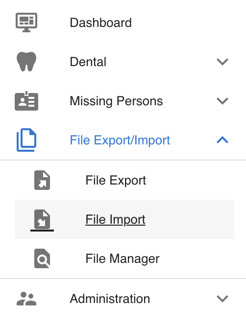
Import File
Using the correct template for importing data is important, CoRA makes it easy to ensure your existing files match files that system will accept without error.
- Select the drop down
- Select the file type you would like to import
- Upon selecting the file template you would like to import, a sample of the file will be downloaded to your computer. Use this sample template to ensure that the information you are importing will be accepted without error.
- You will then be able to upload the file you want into the system.
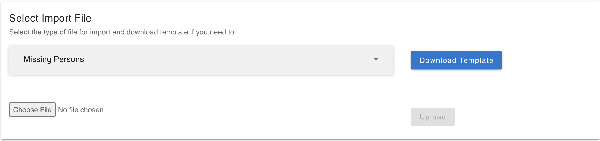
Once the file you wish to import is in the correct format, you may import the file into the system.
- Select "Choose File"
- Choose the correct file from your system's file explorer
- Select "Upload"
Your file will now be uploaded into the system and updates will be made.
Missing Person Dashboard
For more information see the: Missing Person Dashboard User Guide.
Tags
Tags are used to organize and categorize, specimens and DNA samples, allowing for efficient data retrieval and analysis. By associating relevant attributes with each specimen or DNA sequence, tags facilitate tracking, filtering, and sharing of data across research workflows.
Currently Tags can be created of the following types:
- Specimen
- DNA
- Isotope
- Media
Create Tags
Create Tags via Specimen
Tags can be created and assigned to individuals skeletal elements using the Specimen Screen. Follow the steps below to do it:
-
Navigate to the Specimen edit screen:
-
It display multiple sections for modifications.
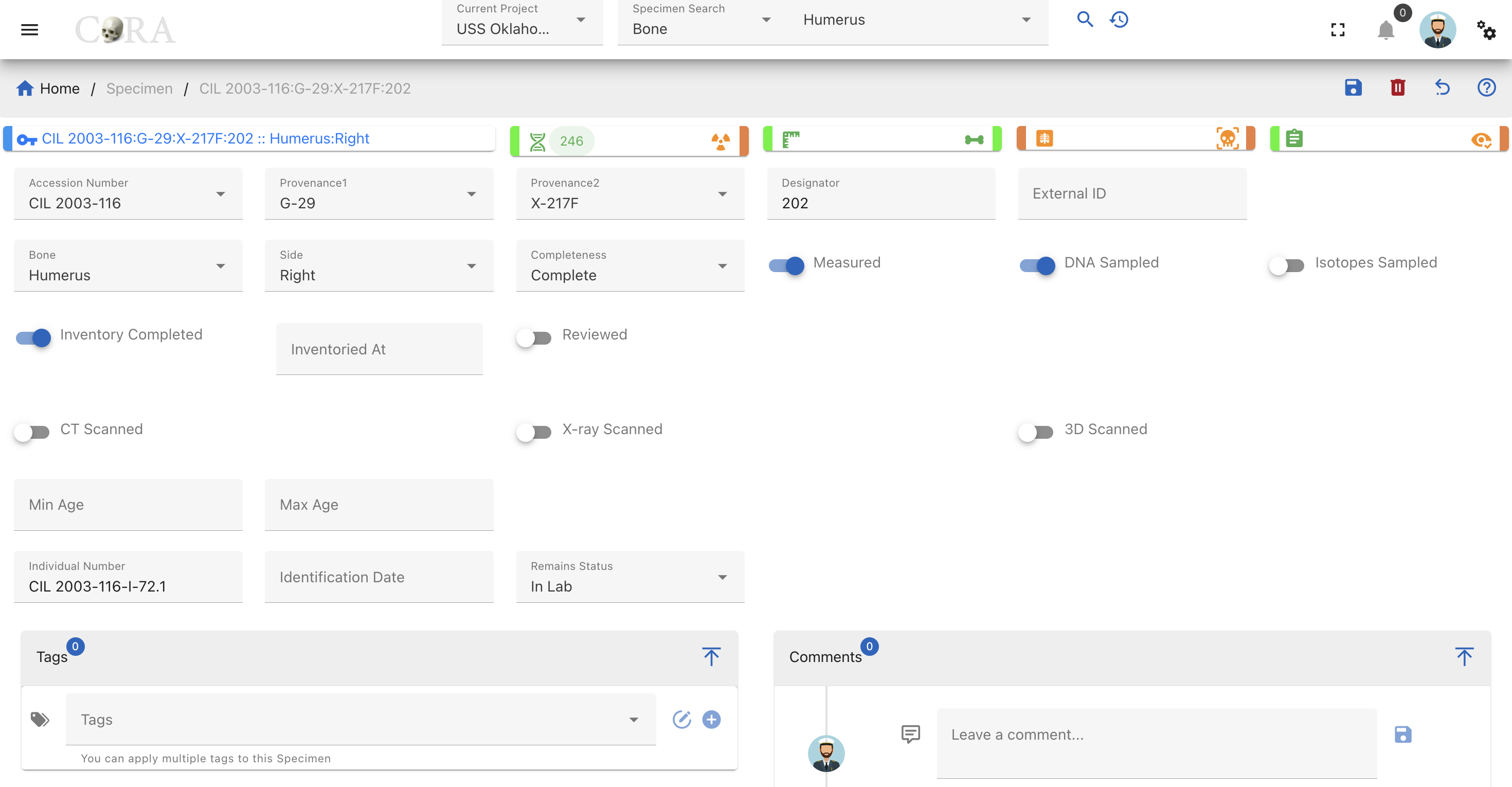
for example you can locate the specimen as below:
-
Navigate to the Tags Section and Create a New Tag:
-
Scroll down to find the Tags section on the editing page. Here, you will see options like Save, Reset/Undo, New, and a dropdown for selecting tags.
- Click the New button to open the Create New Tag dialog box. Enter the required and optional information for the tag:
| Field | Description | Required/Optional |
|---|---|---|
| Tag Name | Name for the tag (letters and numbers, max 32 chars) | Required |
| Description | Brief description (alphanumeric, max 255 chars) | Required |
| Category | Specify the category (letters and numbers, max 32 chars) | Required |
| Type | Define the type of tag (letters and numbers, max 32 chars) | Required |
| Color | Hex code for the tag color | Required |
| Icon | Material Design Icon (mdi) code for visual representation | Required |
- After entering all required and optional details, click Save. A success message, \"Tag successfully added,\" will appear at the top of the screen.
-
Assign the Tag and Save Changes:
-
In the Tags section, select the newly created tag (or an existing one) from the dropdown menu.
- Attach it to the skeletal element.
- Click Save on the editing page to finalize the changes. A confirmation message will indicate that the tag has been successfully assigned to the specimen.
Create Tags Through DNA
Tags can be created and assigned to individuals skeletal elements using the DNA Screen. Follow the steps below to do it:
-
Navigate to the DNA edit screen:
-
It display multiple sections for modifications.
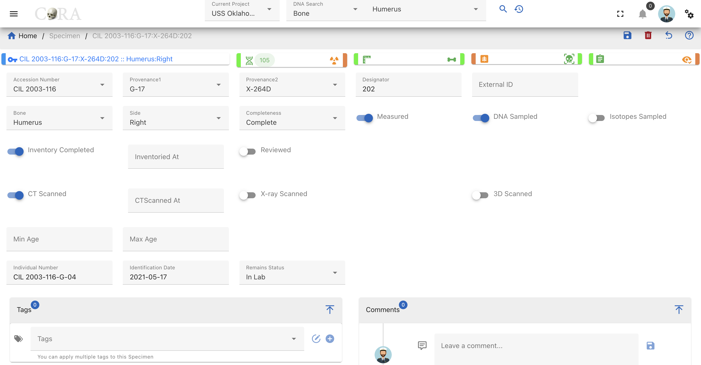
for example you can locate the DNA as below:
-
Navigate to the Tags Section and Create a New Tag:
-
Scroll down to find the Tags section on the editing page. Here, you will see options like Save, Reset/Undo, New, and a dropdown for selecting tags.
- Click the New button to open the Create New Tag dialog box. Enter the required and optional information for the tag:
| Field | Description | Required/Optional |
|---|---|---|
| Tag Name | Name for the tag (letters and numbers, max 32 chars) | Required |
| Description | Brief description (alphanumeric, max 255 chars) | Required |
| Category | Specify the category (letters and numbers, max 32 chars) | Required |
| Type | Define the type of tag (letters and numbers, max 32 chars) | Required |
| Color | Hex code for the tag color | Required |
| Icon | Material Design Icon (mdi) code for visual representation | Required |
- After entering all required and optional details, click Save. A success message, "Tag successfully added," will appear at the top of the screen.
-
Assign the Tag and Save Changes:
-
In the Tags section, select the newly created tag (or an existing one) from the dropdown menu.
- Attach it to the skeletal element.
- Click Save on the editing page to finalize the changes. A confirmation message will indicate that the tag has been successfully assigned to the specimen.
Search via tags
Specimen Search via Tags
Users can search for specimen which are associated with the particular tag in the application using the Specimen Search functionality.
-
Navigate to Specimen Search:
-
Locate the Tags dropdown on the application interface.
-
Select Tags:
-
Open the tags dropdown menu and select the tag for which you need the associated specimens.
-
Search and View Results:
-
Hit the Search button to execute the query.
- A results sheet will be displayed, showing the selected specimens for the selected tag.
DNA Search via Tags
Tag Management
The Org Administrator has the ability to browse tags list, create and manage the tags along with the ability to assign tags to projects and Organizations. The tags management screen provides a data table of all the tags in the current organization with information such as Name, Description, Category, Type, Color, and Icon. The tags list will be initially sorted on the name. The data table also has an Actions column with buttons to edit the tag.
tip
- You can edit the tag by clicking the name link.
- The column visibility will allow you to add more columns/details to the data table list.
- The Search box can be used to search any details in the data table list.
Create Tag from Tag Management
On the tag management screen, click the Create button/icon to create a new tag. Navigation to the tag management screen is shown below.
The Create button opens a dialog box to prompt to create a new tag. Enter the information for the new tag record.
Once all information is entered, click Save, and a success message Tag successfully added will appear at the top.
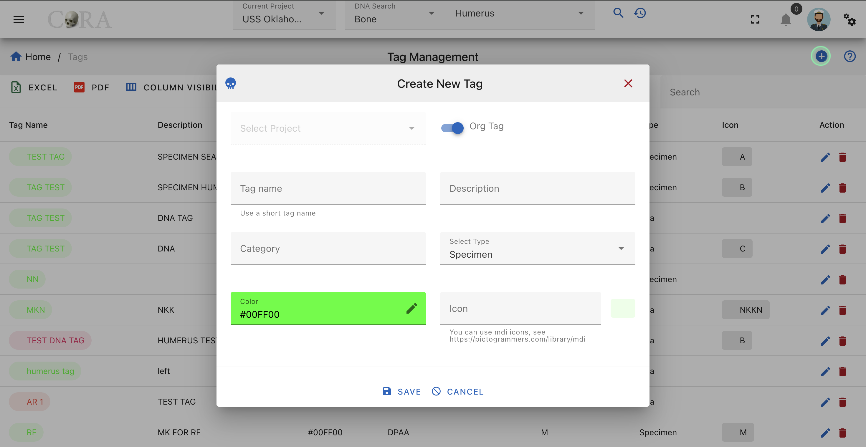
Screen Fields
Fields in bold are required.
| Attributes | Data Type | Size | Validation Rule | Required/Optional |
|---|---|---|---|---|
| Project | Id | valid option via dropdown | Required (Default current project) | |
| Tag Name | String | 32 chars | contains letters and numbers | Required |
| Description | String | 255 chars | contains alphanumeric | Required |
| Category | String | 32 chars | contains letters and numbers | Optional |
| Type | String | 32 chars | contains letters and numbers | Optional |
| Color | String | 32 chars | color hex number | Optional |
| Icon | String | 32 chars | mdi icon (see material design icon codes) | Optional |
Edit Tag
To edit an existing tag information, simply click on the Name, and the edit dialog box will open for editing the existing tag information. The following fields are available for update. Click Save when finished editing, or Close to cancel the changes.
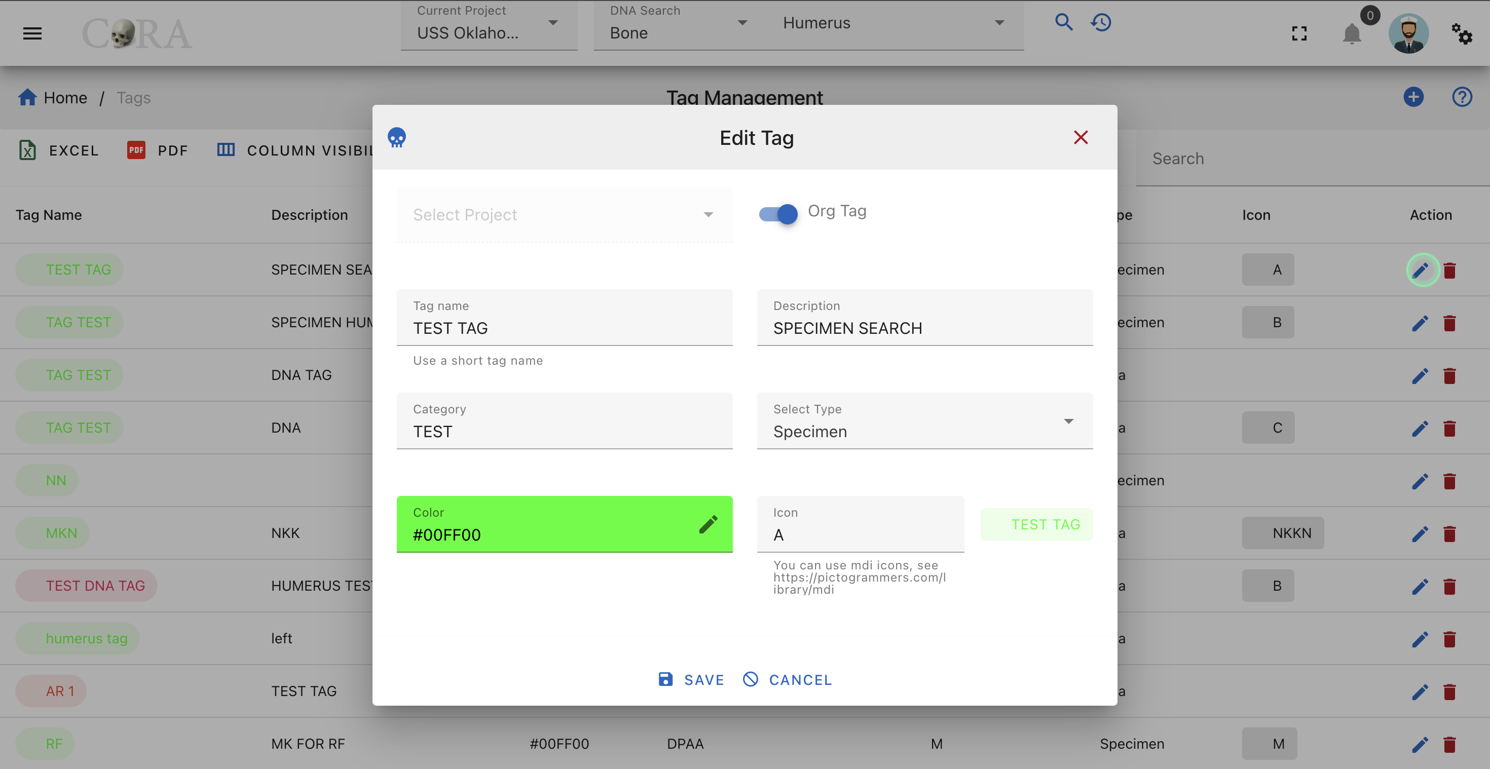
Screen Fields
Fields in bold are required.
| Attributes | Data Type | Size | Validation Rule | Required/Optional |
|---|---|---|---|---|
| Project | Id | valid option via dropdown | Required (Default current project) | |
| Tag Name | String | 32 chars | contains letters and numbers | Required |
| Description | String | 255 chars | contains alphanumeric | Required |
| Category | String | 32 chars | contains letters and numbers | Optional |
| Type | String | 32 chars | contains letters and numbers | Optional |
| Color | String | 32 chars | color hex number | Optional |
| Icon | String | 32 chars | mdi icon (see material design icon codes) | Optional |
Delete Tag
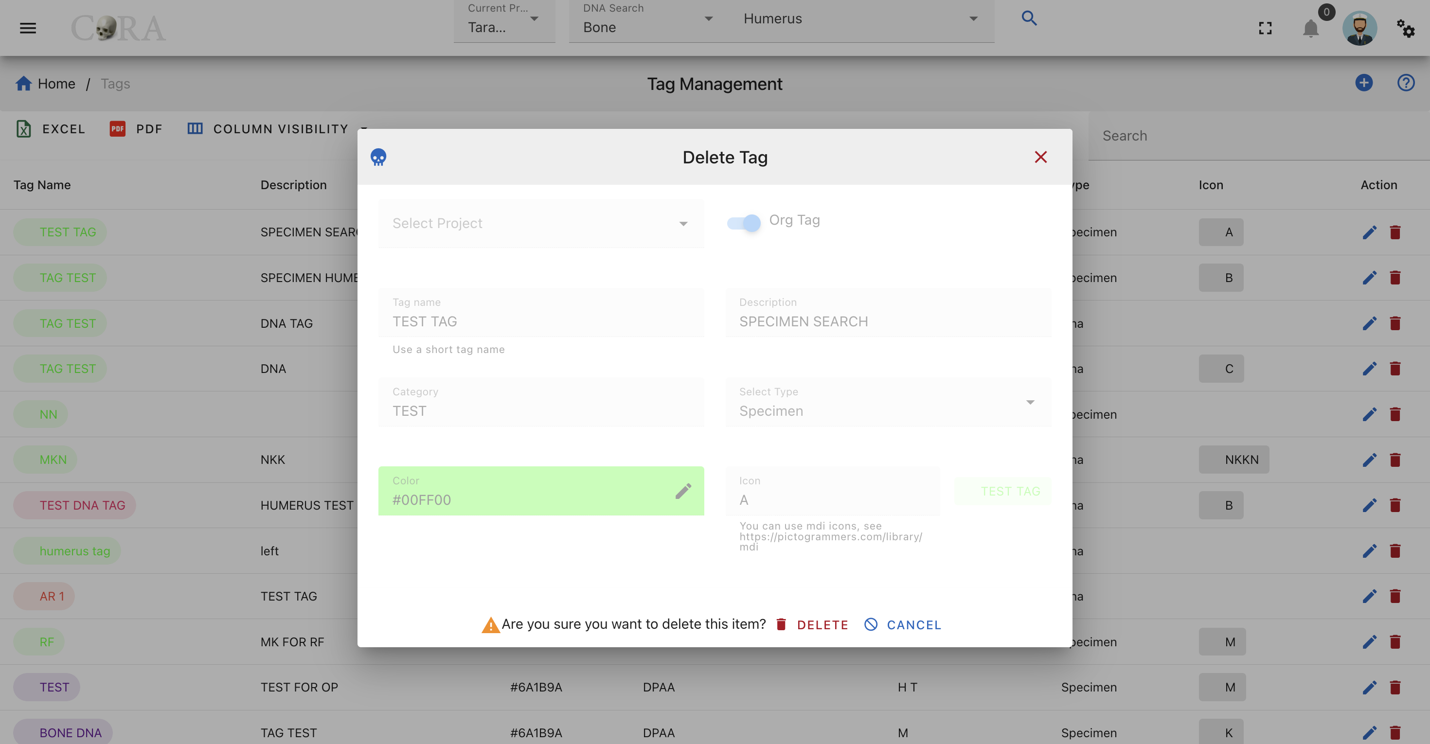
Moving Project tags to Org tags
If particular tag is required at organization level, it can be moved from project level to Org level.
Search
Search
CoRA provides a powerful search engine allowing you to search any modules such as Specimens, DNA, Isotopes, Dental, Missing Persons. Each module can be searched using multiple criteria which are related to that module.
Search History and Favorites
The search capability also comes with a search history and favorites, which allows the user to look at their search history and create favorites from their search history. This allows the user to quick access previous searches they may have done in a project.

The searched type can be added to favorites. By clicking on the favorites from the history tab.

To delete the favorites history from favorites tab click on delete

Quick Search
The quick search capability in CoRA is available in the header. It has 3 main components, the project, the search module, search criteria.
Project Selector
The project selector displays the current project that the user is working on and all searches are done within the context of the currently selected project. You can change your project anytime you want via the project dropdown by selecting a different project.
Module Selector
The module or model selector displays the models that the user can search along with the most frequently used criteria for that model. You can change your model criteria anytime you want via this dropdown.
Search String/Value
The search string or value is provided by the user by either typing the search string or selecting a value from a the dropdown.
The values in the dropdown will change based on the module selected iby the user. CoRA has a built in intellisense engine that will provide
the user with the most appropriate or valid search options for the selected project and module.
Intellisense Engine
CoRA has a built in intellisense engine that will provide context sensitive information, options and values for the selected project and model.
Search by Specimen
The user can search by the below Specimen search options under the Specimen Section in the search dropdown. Below you will see some examples of how to complete searches.
Specimen Search Options:
- Bone
- External Specimen ID
- Composite Key
- Accession
- Provenance 1
- Provenance 2
- Designator
- Individual Number
- Tags
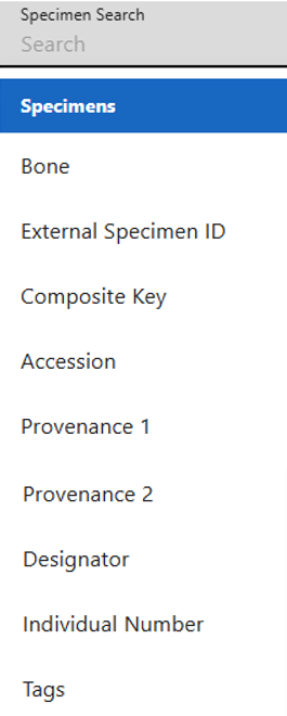
Bone
With the Bone option, an user can search specimens by selecting a bone name. As seen in the image above, user can search for the specimen by the bone names such as Humerus, Tiba etc. The SE eg Humerus, Tibia, Cranium indicates you are searching for the Skeletal elements either by bone Humerus or Tiba or Cranium etc. At one time, you can only search for one bone name in this search category.

- Make sure you are on the project you want to search the specimen in.
- Under the Specimen Search select the 'Bone' option.
- Then select the bone you would like to search for.
- Next click on the magnifying glass search icon to show the search results.
Below is the search result obtained from specimen search by bone 'Accessory Rib'.

External Specimen ID
With the 'External Specimen ID' option, the user can search specimens by typing in the 'External Specimen ID'.

- Make sure you are on the project you want to search the specimen in.
- Under the Specimen Search select the 'External Specimen ID' option.
- Then enter in the 'External Specimen ID' (e.g. 333.1).
- Next click on the magnifying glass search icon to show the search results.
Search results by External Specimen ID equal to 333.1.
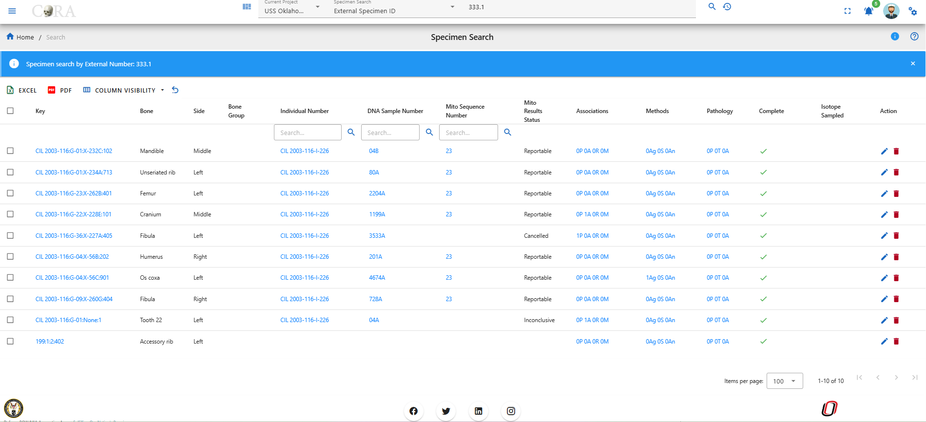
Composite key
When searching by composite key, use the comma separator "," to differentiate between accession number, provenance1, provenance2 and designator fields.

- Make sure you are on the project you want to search the specimen in.
- Under the Specimen Search select the 'Composite key' option.
- Then enter in the 'Composite key' (includes key of specimen, accession number, provenance1, provenance2, designator, etc, fields).
- Next click on the magnifying glass search icon to show the search results.
Below is the search result obtained from specimen search by composite key 'CIL 2003-116,G-03,,,712'.
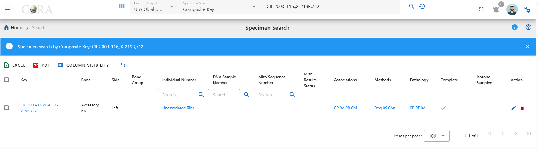
The pattern for the composite search is 'Accession,Provenance1,Provenance2,Designator'. If any of fields are not there or if you want to skip some fields, then you can keep the fields empty and use the comma separator.
For example, in the below search criteria, we do not have Provenance 2. So we can lookup for the specimens with accession number, provenance 1 and designator with empty field for provenance 2 with ',' separator. CIL 2003-116,,X-219B,712
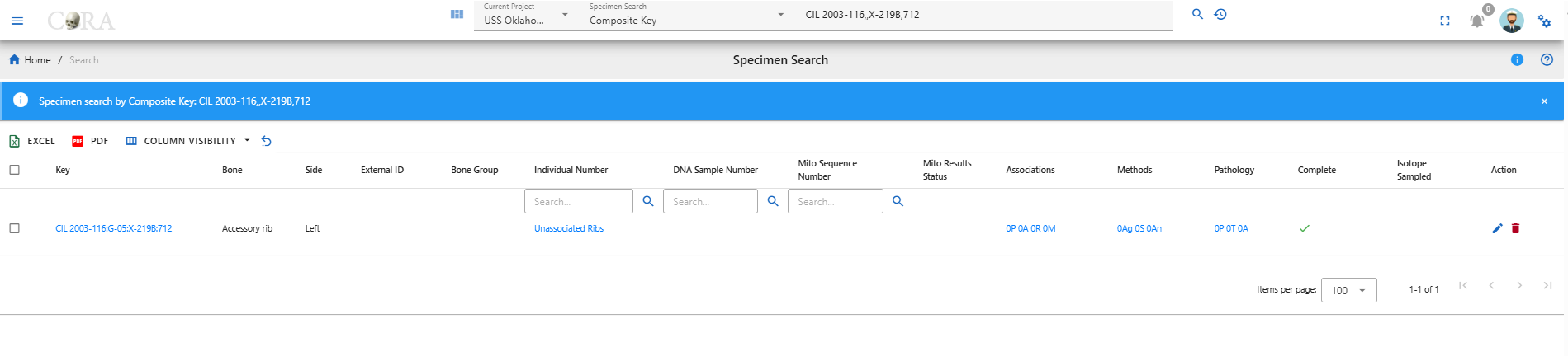
Similarly, in the screenshot below you can see we have excluded provenance 1 and provenance 2 from our search but have kept the comma separator for them.
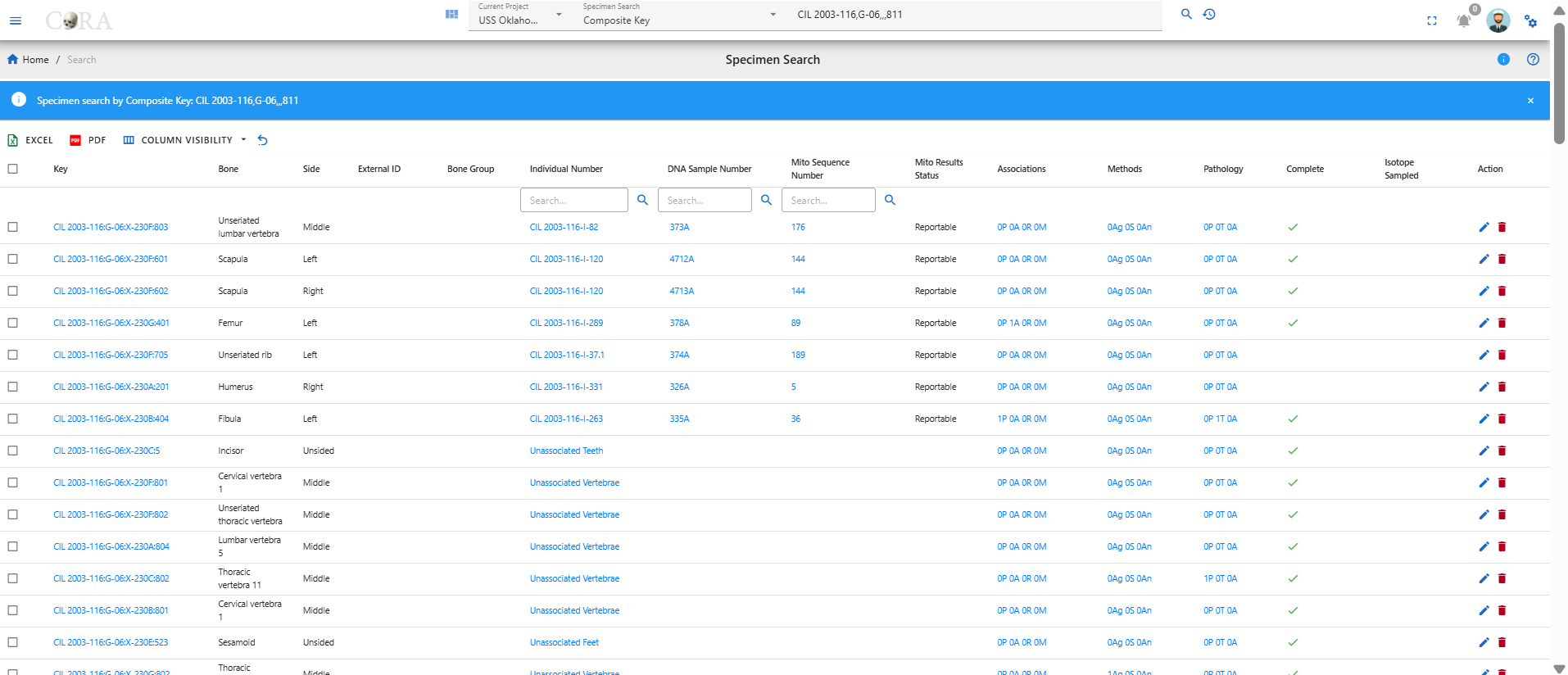
Accession
With the Accession option, the user can search specimens by choosing the their Accession number from the drop down menu. A user can search for the specimen from the Accession numbers such as 'CIL 2003-116', 'CIL 2018-337' etc, a drop down list of available accession numbers will appear.At one time, you can only search for one accession number in this search category.
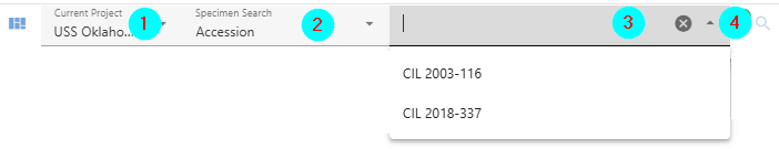
- Make sure you are on the project you want to search the specimen in.
- Under the Specimen Search select the 'Accession' option.
- Then from the drop down select the accession number you would like to search for.
- Next click on the magnifying glass search icon to show the search results.
Below is the search result obtained from specimen search by Accession number 'CIL 2003-116'.
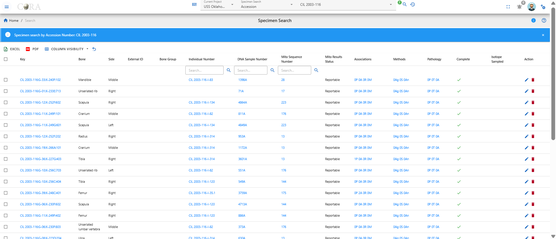
Provenance 1
With the Provenance 1 option, the user can search specimens by writing their Provenance 1. As seen in the image above, user can search for the specimen by providing the Provenance 1 such as G-21, G-212 etc. The SE eg G-21 0r G-212 indicates you are searching for the Skeletal elements either by Provenance 1 'G-21' or 'G-212' At one time, you can only search for one Provenance 1 in this search category. Below is the search result obtained from specimen search by Provenance 1 'G-57E'.
Provenance 2
With the Provenance 2 option, the user can search specimens by writing their Provenance 2. As seen in the image above, user can search for the specimen by providing the Provenance 2 such as X-1 etc. The SE eg X-1 0r Trench 3 indicates you are searching for the Skeletal elements either by Provenance 2 'X-1' or 'Trench 3' At one time, you can only search for one Provenance 2 in this search category. Below is the search result obtained from specimen search by Provenance 2 'X-299C'.
Designator
With the Designator option, the user can search specimens by writing their Designator. As seen in the image above, user can search for the specimen by providing the Designator such as 201, 602 etc. The SE eg 201 or 602 indicates you are searching for the Skeletal elements either by Designator '201' or '602'. At one time, you can only search for one Designator in this search category.
Individual Number
With the Individual Number option, the user can search specimens by writing their Individual Number. As seen in the image above, user can search for the specimen by providing the Individual Number such as I-01 etc. While searching for the specimen using individual number, one has to add its Accession number together with the individual. For example, in order to search for the specimen having I-01 individual number one has to type '2016-235-I-01' or 'CIL 2003-116-I-01'. At one time, you can only search for one Individual Number in this search category.
Tags
With the Tags option, the user can search specimens by their Tag from the dropdown. As seen in the image above, user can search for the specimen by providing the Tag such as "Specimen".
At one time, you can select multiple Tags to search by in this search category.
Search by DNA
The user can search by the below DNA search options under the DNA Section in the search dropdown. The DNA search options are similar to the Specimen search options.
DNA Search Options:
- Bone
- Composite Key
- Accession
- Provenance 1
- Provenance 2
- Designator
- Sample Number
- Mito Sequence Number
- External Case ID
- External Sample Number
- Tags

Sample Number
With the Sample Number option, the user can search DNA by their Sample numbers. As seen in the image above, user can search for the DNA by the sample numbers such as 68A or 4619A. The DNA eg 68A or 4619A indicates you are searching for the DNA either by sample numbers '68A' or '4619A' etc. At one time, you can only search for one sample number in this search category.

- Make sure you are on the project you want to search in.
- Under the DNA Search select the 'Sample Number' option.
- Then type in the sameple number you would like to search for.
- Next click on the magnifying glass search icon to show the search results.
Below is the search result obtained from DNA search by sample number '68A'.
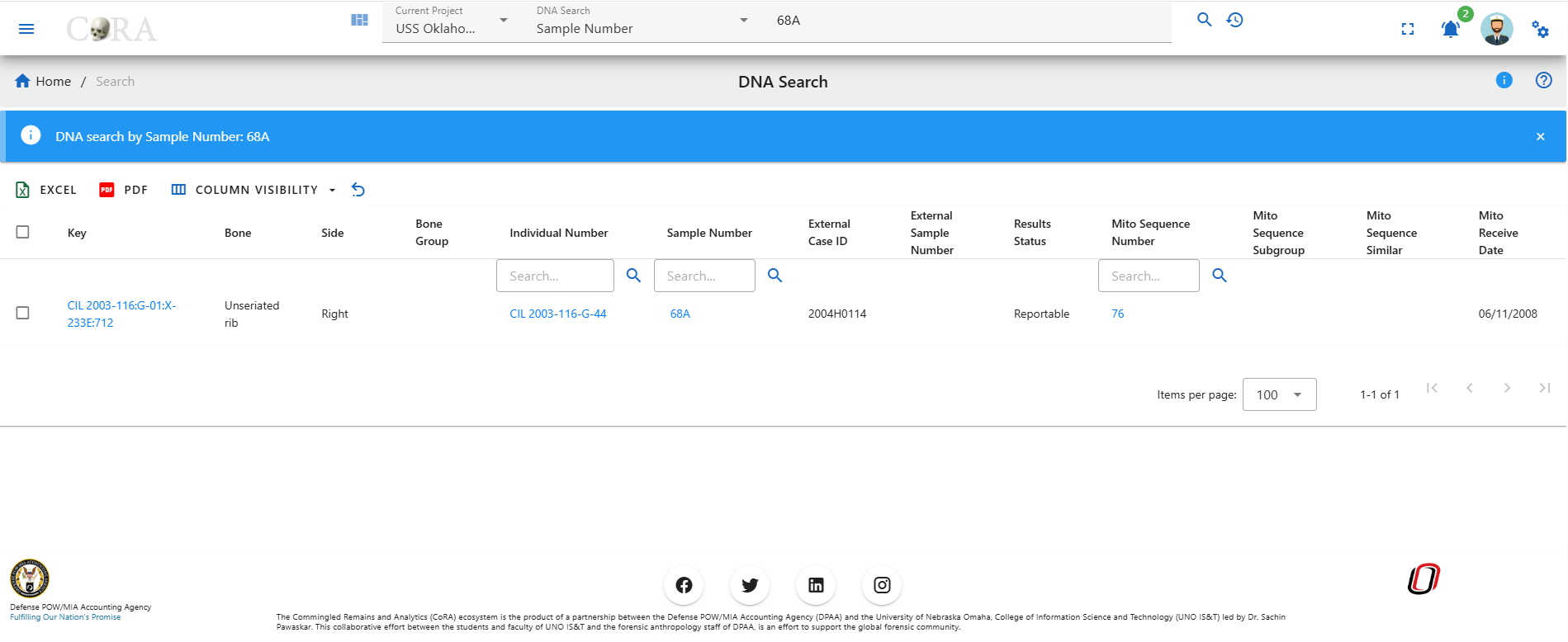
Mito Seq Number
With the Mito Seq Number option, the user can search DNA by their Mito Seq Numbers. As seen in the image above, user can search for the DNA by the Mito Seq Number such as 1 or 76. The DNA eg 1 or 76 indicates you are searching for the DNA either by mito seq numbers '1' or '76' etc. At one time, you can only search for one mito seq number in this search category.

- Make sure you are on the project you want to search in.
- Under the DNA Search select the 'Mito Seq Number' option.
- Then type in the mito seq number you would like to search for.
- Next click on the magnifying glass search icon to show the search results.
Below is the search result obtained from DNA search by mito seq number '76'.
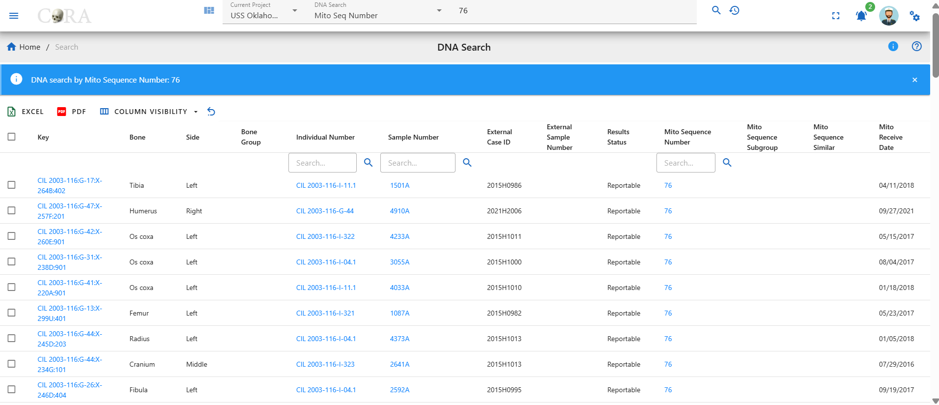
External Case ID
With the External Case ID option, the user can search DNA by their External IDs. As seen in the image above, user can search for the DNA by the External ID such as 2004H201 or 2015HO860. The DNA eg. AFDIL # like 2004H2001 or 2015HO860 indicates you are searching for the DNA either by external id '2004H2001' or '2015HO860' etc. In order to search for the DNA, you just have to give the external id without the lab name as shown below.
At one time, you can only search for one external case id in this search category.

Below is the search result obtained from DNA search by external id '2015H1002'.
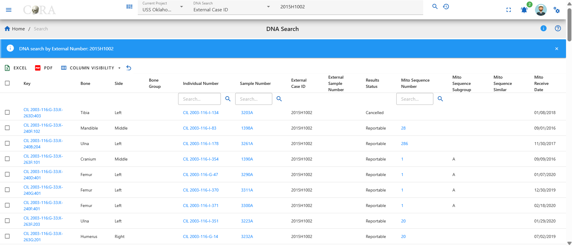
Search by Isotope
The user can search by the below Isotope search options under the Isotope Section in the search dropdown. The options are similar to the Specimen and DNA searh options.
Isotope Search Options:
- Bone
- Composite Key
- Accession
- Provenance 1
- Provenance 2
- Designator
- Sample Number
- Tags
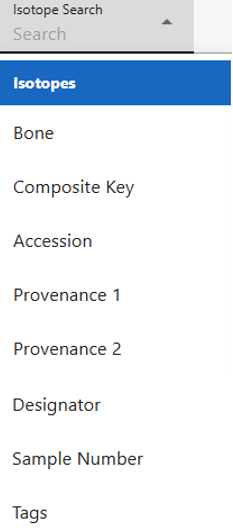
Sample Number
With the Sample Number option, the user can search Isotopes by a Sample number. As seen in the image above, user can search for the Isotope by the sample numbers such as 38B.
The Isotope eg 38B indicates the user is searching for the Isotope by sample number. At one time, the user can only search for one sample number.
Below is the search result obtained from DNA search by sample number '38B'.
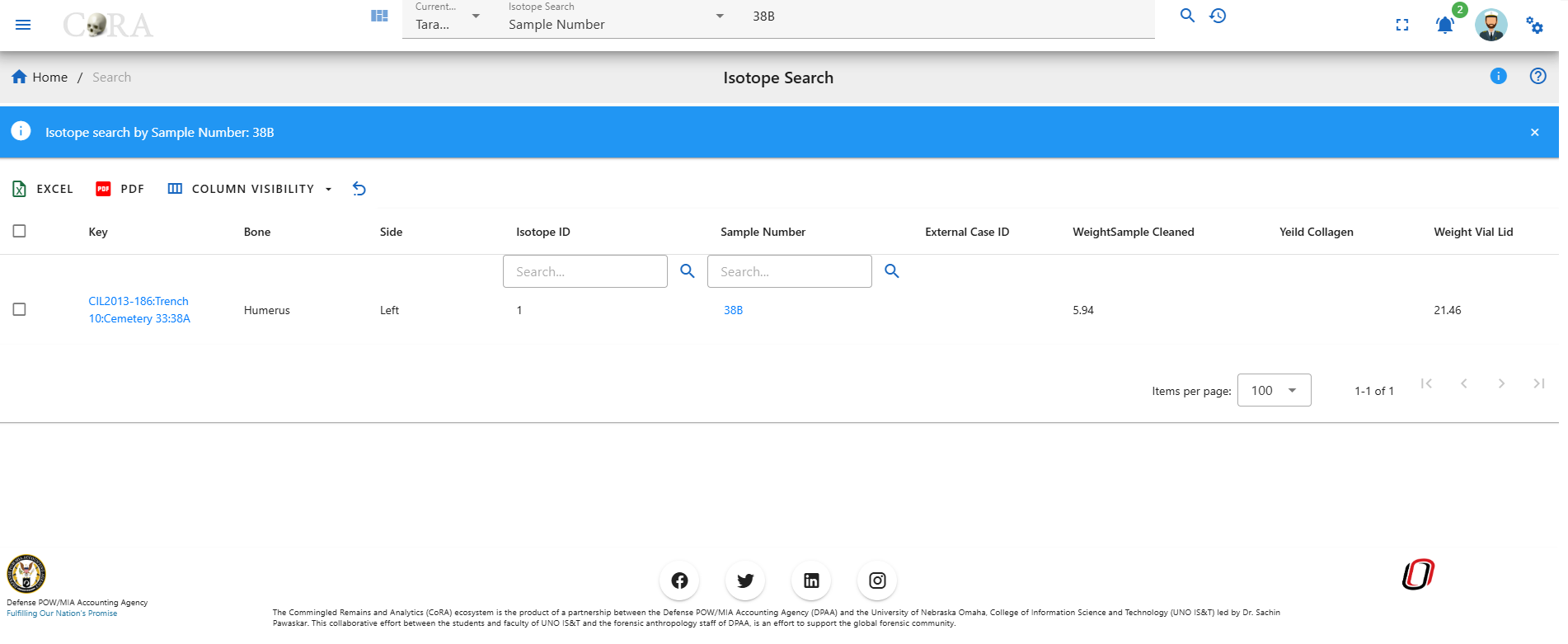
Search by Dental
The user can search by the below Dental search options under the Dental Section in the search dropdown.
Dental Search Options:
- Tooth
- Dental Code
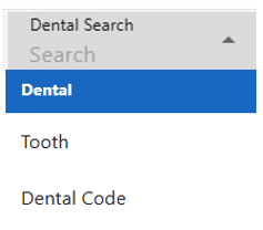
Tooth
!!! This section is a work in progress
Dental Code
!!! This section is a work in progress
Search by Missing Person
The user can search by the below Missing Person search options under the Missing Person Section in the search dropdown.
Missing Person Search Options:
- Case Manager
- Case Status
- Conflict
- Genealogy Status
- First Name
- Last Name
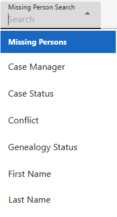
Case Manager
With the Case Manager option, the user can select different case managers associated under the project and click on the search button will display missing person details under that selected case manager.
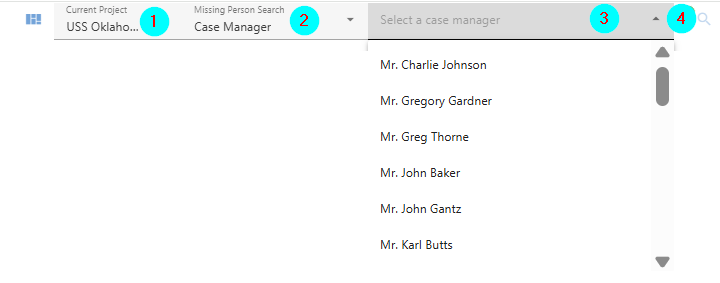
- Make sure you are on the project you want to search the missing person in.
- Under the Missing Person Search select the 'Case Manager' option.
- Then from the drop down select the name of the case manager you would like to search for.
- Next click on the magnifying glass search icon to show the search results.
Below displays missing person details assigned for case manager named as Mr. Charlie Johnson
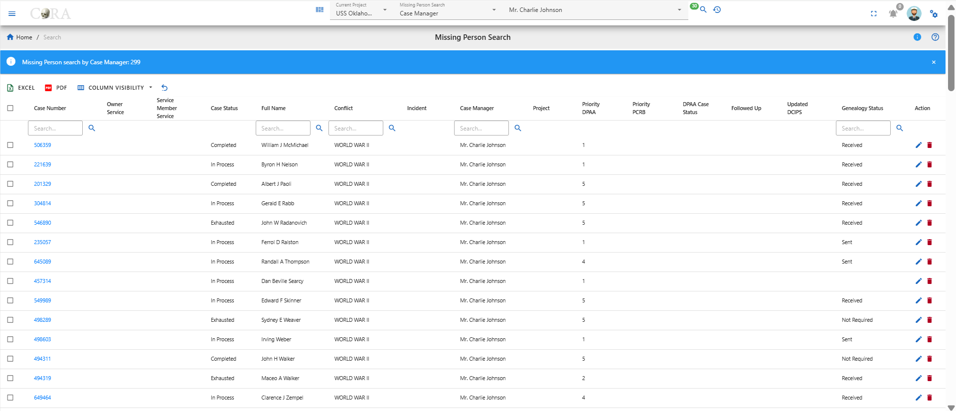
Case Status
With the Case Status option, the user can select different case status associated under the project and click on the search button will display missing person details under that selected case status.
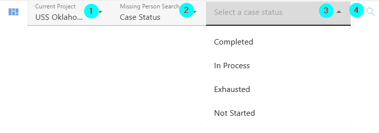
- Make sure you are on the project you want to search the missing person in.
- Under the Missing Person Search select the 'Case Status' option.
- Then from the drop down select the case status you would like to search for.
- Next click on the magnifying glass search icon to show the search results.
Below displays missing person details whose case status is completed.

Conflict
With the Conflict option, the user can select different Conflict associated under the project and click on the search button will display missing person details under that selected conflict.
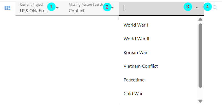
- Make sure you are on the project you want to search the missing person in.
- Under the Missing Person Search select the 'Conflict' option.
- Then from the drop down select the conflict you would like to search for.
- Next click on the magnifying glass search icon to show the search results.
Below displays missing person details assigned to conflict named World War I.
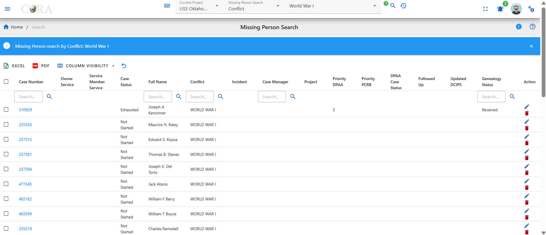
Genealogy Status
With the Genealogy Status option, the user can select different Genealogy status associated under the project and click on the search button will display missing person details under that selected genealogy status.
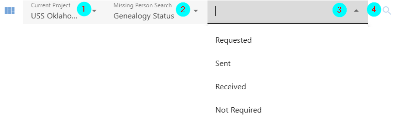
- Make sure you are on the project you want to search the missing person in.
- Under the Missing Person Search select the 'Genealogy Status' option.
- Then from the drop down select the genealogy status you would like to search for.
- Next click on the magnifying glass search icon to show the search results.
Below displays missing person details of genealogy status as requested.
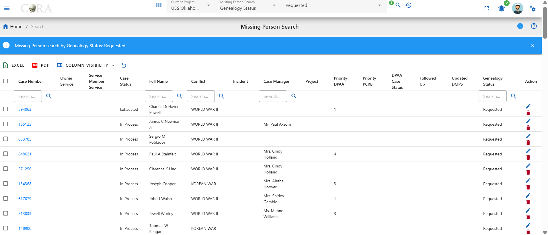
First and Last Name
With the First/Last Name option, the user can search for different case numbers associated with the given first/last name under a project and click on the search icon will display missing person details for that selected first/last name.
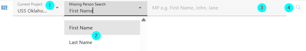
- Make sure you are on the project you want to search the missing person in.
- Under the Missing Person Search select the 'First or Last Name' option.
- Then type in the first or last name you would like to search for.
- Next click on the magnifying glass search icon to show the search results.
Below displays missing person details of first name as Charlie
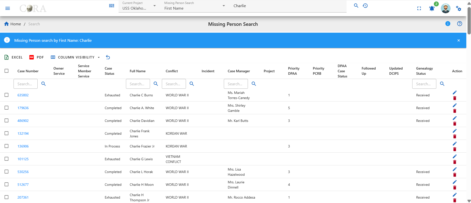
Search by Individuals
The user can search by the below Individuals search options under the Individuals Section in the search dropdown.
Individuals Search Options:
- Individual Number
- Identification Date
- Remains Status
- Remains Release Date
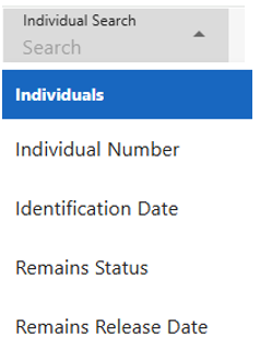
Indentification Date
With the Indentification Date option, the user can search for a range of indentification dates under a project.

- Make sure you are on the project you want to search the missing person in.
- Under the Individual Search select the 'Identification Date' option.
- Then select or type in the start and end dates you would like to search for.
- Next click on the magnifying glass search icon to show the search results.
Below displays the individuals that have an indentification date range of 11/01/2017 - 11/30/2017.
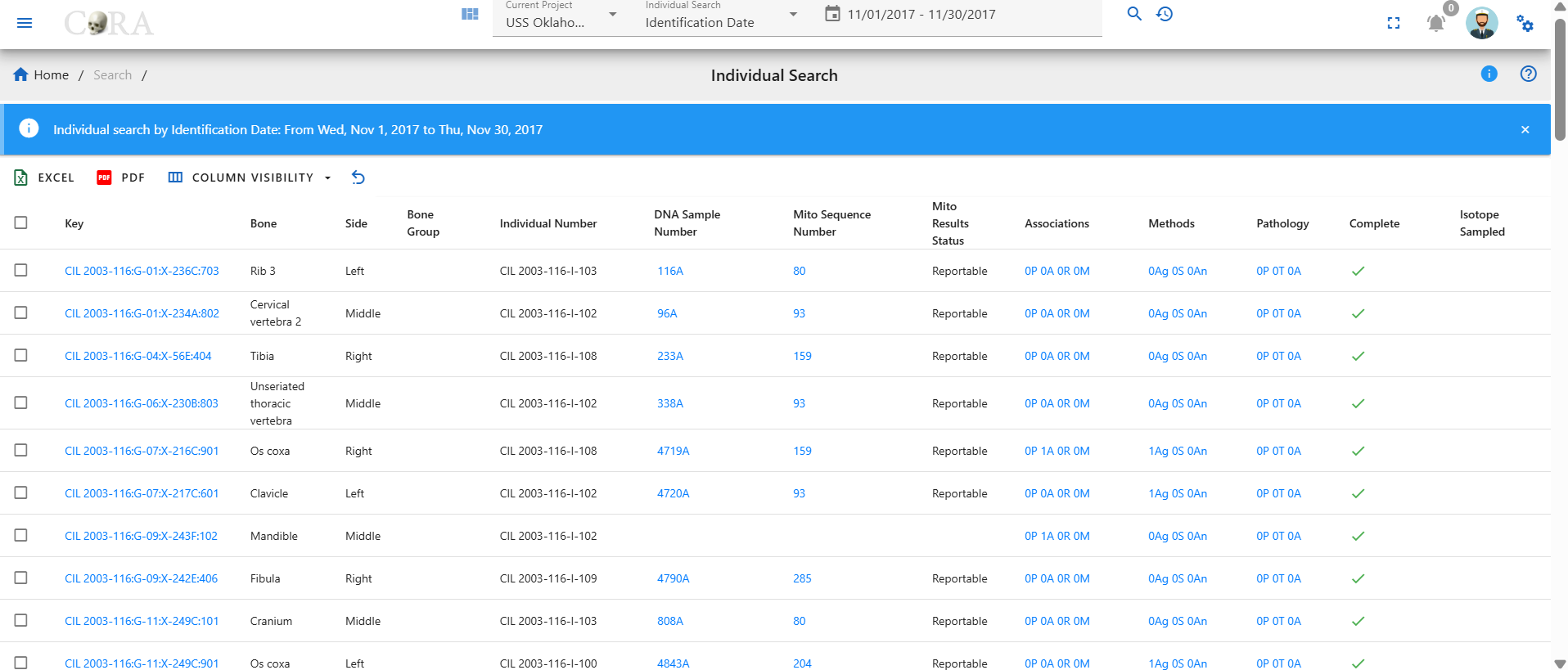
Remains Status
With the Remains Status option, the user can search for a remains status under a project.
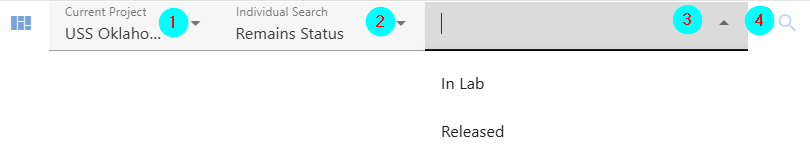
- Make sure you are on the project you want to search the missing person in.
- Under the Individual Search select the 'Remains Status' option.
- Then select the remains status you would like to search for.
- Next click on the magnifying glass search icon to show the search results.
Below displays the individuals that have a remains status of In Lab.
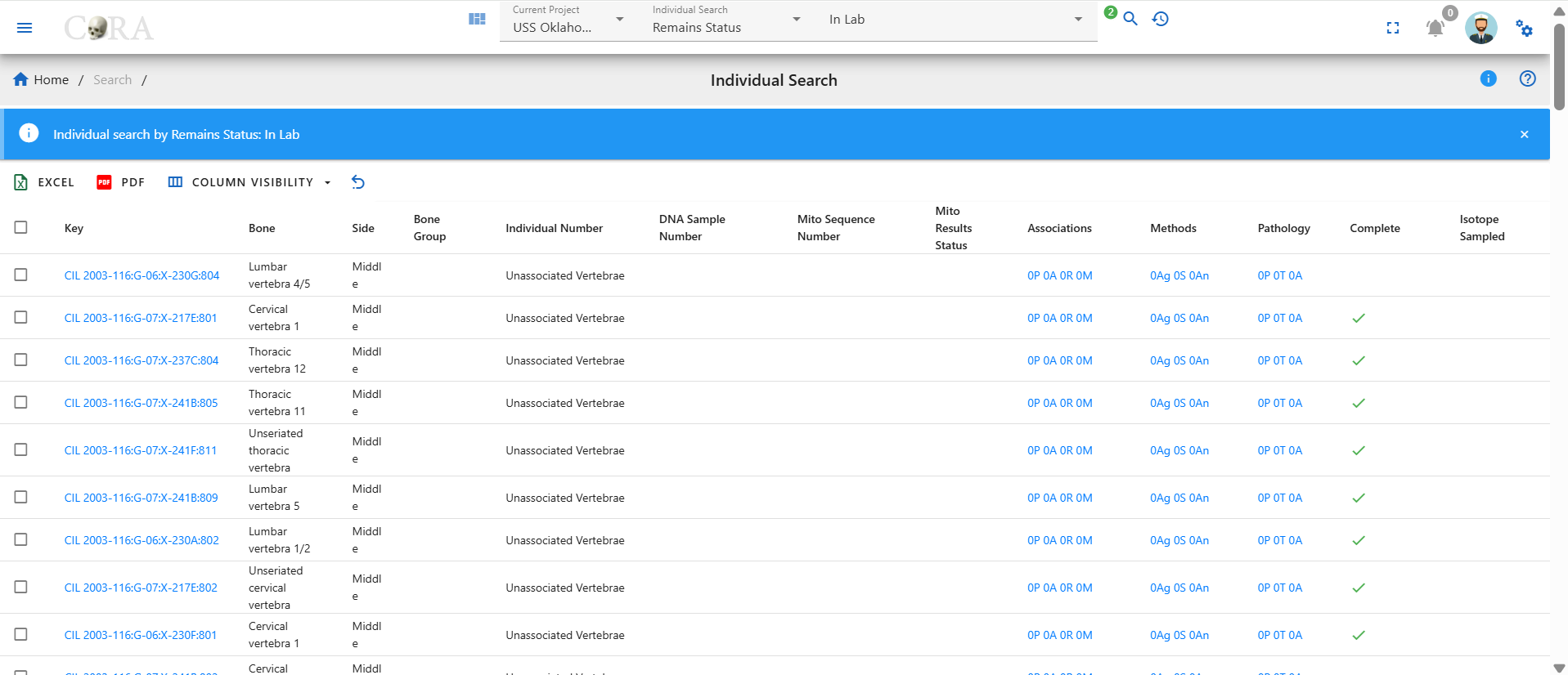
Search Options
Max Search Limit 500
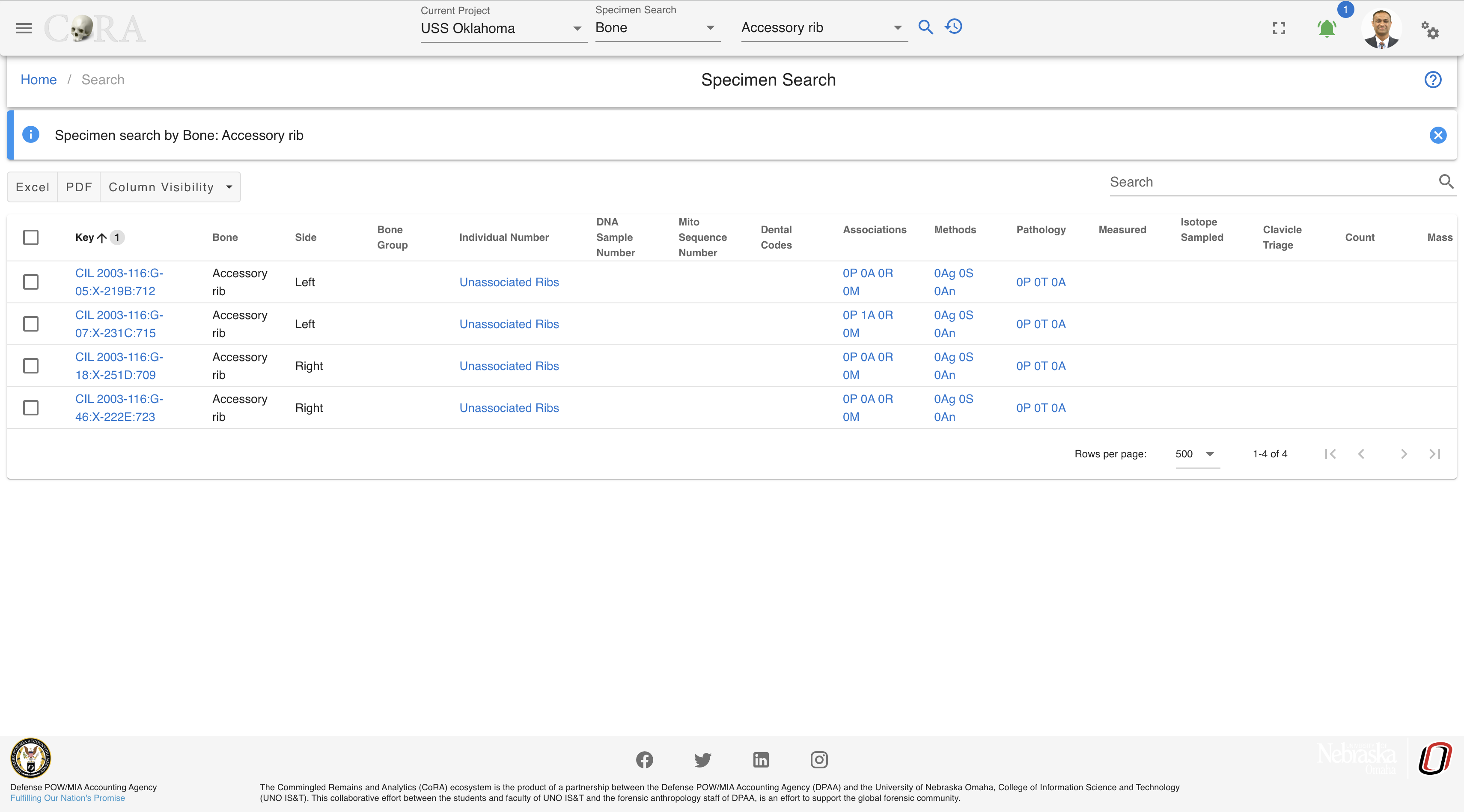 The server renders all results queried from the project search bar request, allowing the user to paginate and search through the entire response. Limitations with this search options, include longer response times or application overload for projects with large sets of data.
Each tab will generate a new call to the server and retrieve the next set of data. This search option is ideal for project with larger sets of data. Search result filter is not available with this option.

Advanced Search & Reporting
Along with the quick search capability CoRA also provides an advanced search and reporting capability via the reports dashboard feature. The reports dashboard has many reports and each report provides the ability to search using multiple search criteria. See the documentation on the reports dashboard
Exporting Data
This guide explains how to export data to Excel or PDF after performing a search or applying filters within the application.
Data Search & Filter
Before exporting the data, ensure that the correct dataset is displayed.
- Use the search bar to locate specific records.
- Apply any necessary filters or sorting options.
- Confirm that the table displays the desired results before exporting.
Export
Ensure all search, filter, and sorting options are applied correctly before exporting.
Excel Export
Follow these steps to download the data in Excel format:
- Locate the Excel Export button in the menu bar above the data table.
- Click on the Excel option.
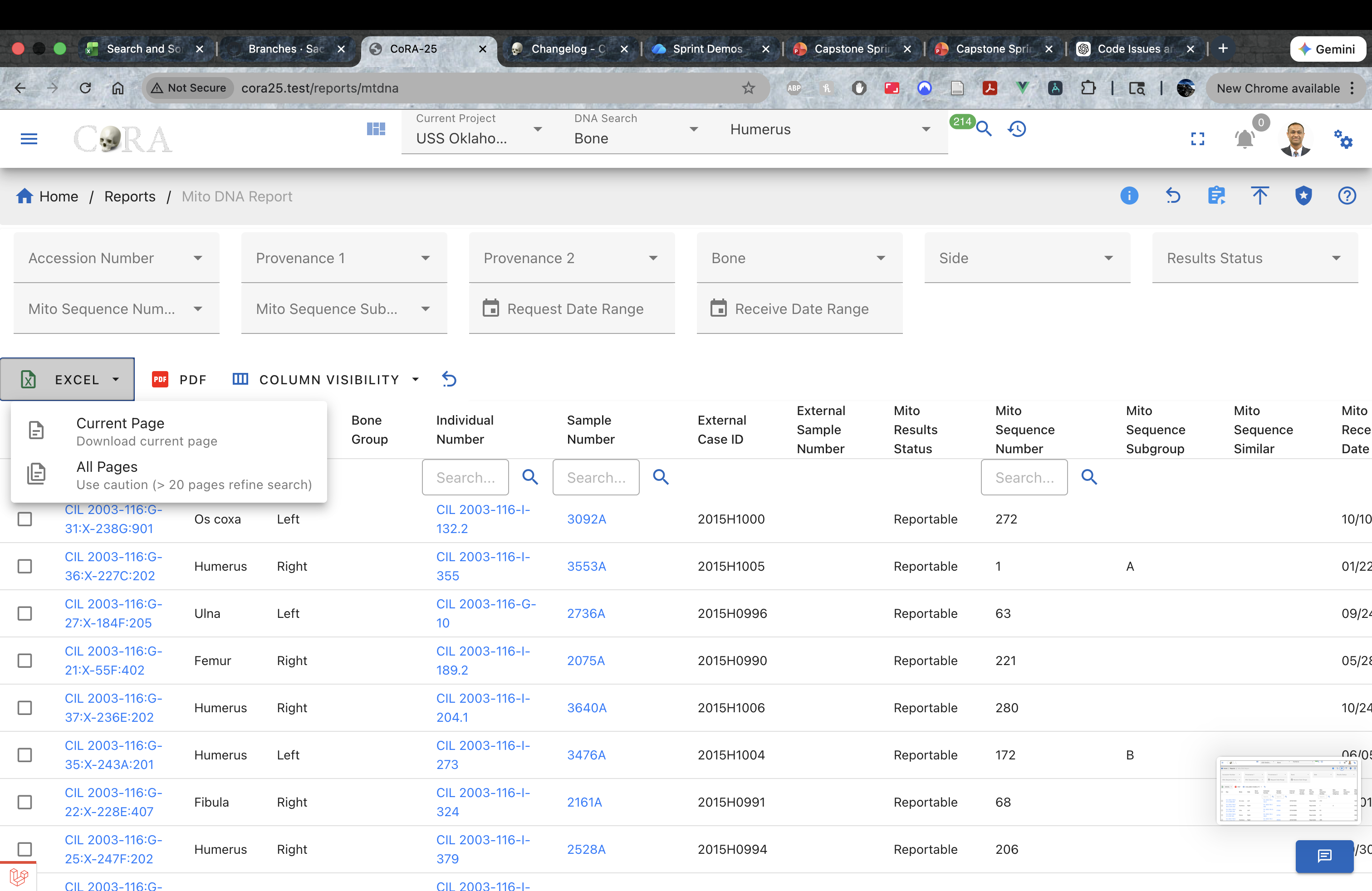
-
After clicking the Excel button, two download options will appear:
-
Current Page – Downloads only the data displayed on the first page of the table.
-
All Pages – Downloads the entire dataset based on the applied search and filter criteria.
-
If All Data is selected, a notification message will appear indicating that the download may take longer depending on the size of the dataset.
-
Once processing is complete, the Excel file will automatically download to your computer.
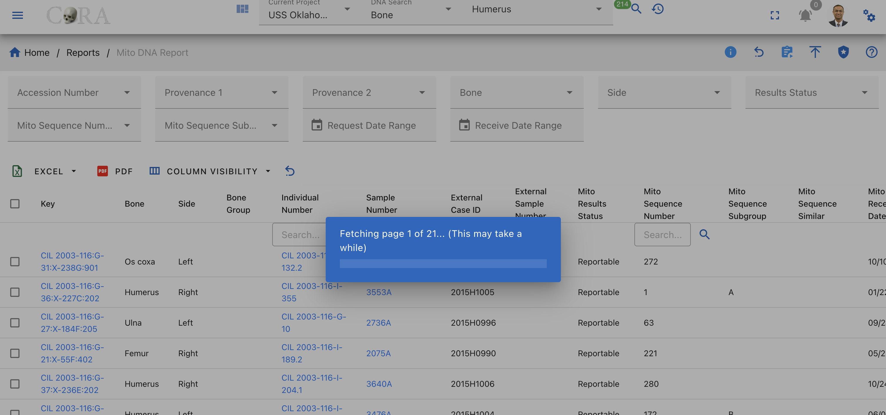
PDF Export
To download the data as a PDF document:
-
Locate the PDF Export button in the menu bar near the Excel export option.
-
Click the PDF button.
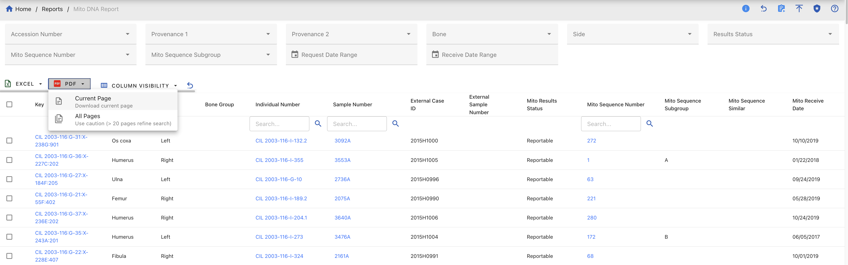
- After clicking the Excel button, two download options will appear:
- Current Page – Downloads only the data displayed on the first page of the table.
- All Pages – Downloads the entire dataset based on the applied search and filter criteria.
-
If All Data is selected, a notification message will appear indicating that the download may take longer depending on the size of the dataset.
-
Once processing is complete, the PDF file will automatically download to your computer.
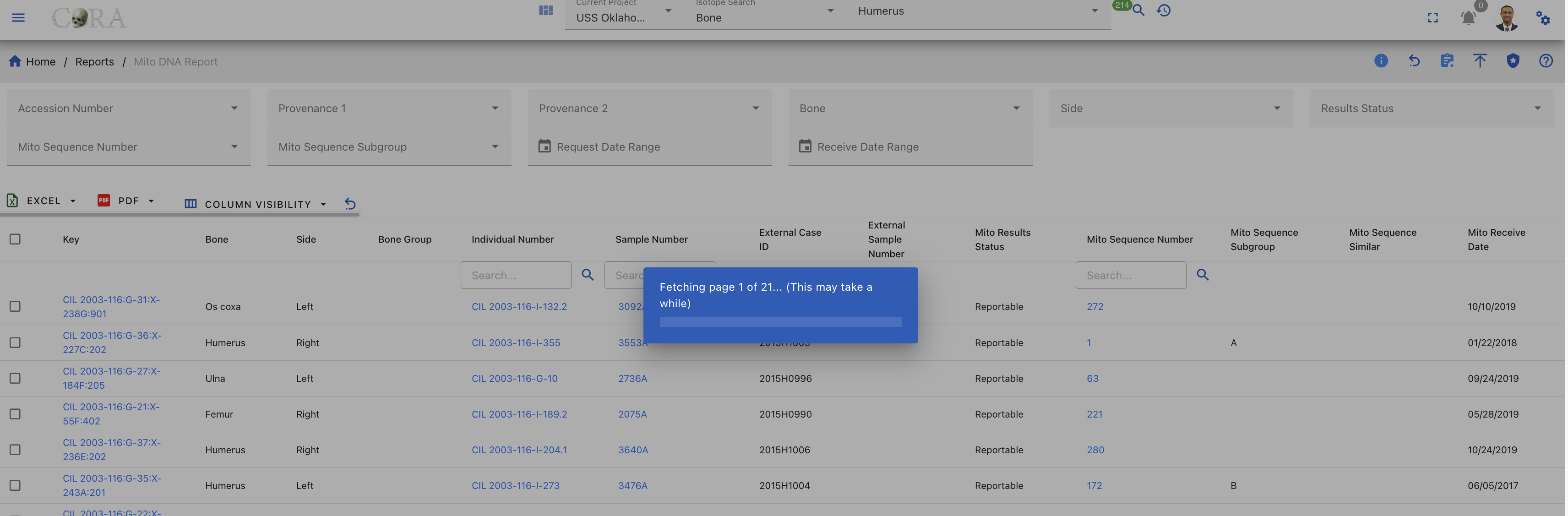
Export All Data Pages
Exporting all data pages may take additional time if the dataset is large. So make sure that you have reduced your search space first before exporting data.
Reports
Reports
Warning
This page is work in progress.
There are three different reports dashboard available in CoRA with each view being driven by the user's profile attributes. 1. The Org Reports 2. The Project Reports 3. The User Reports
Org Reports
This dashboard has a card view listing of all the org reports.
Customize Dashboard
The org reports dashboard is highly customizable. You can expand/collapse all the report tabs or individual tabs and also drag and rearrange the tab arrangement. This arrangement is saved even after the user logs out. This state is saved in your local storage until browser cache is cleared. Each report pane displays an image of its respective sample report showing column names of that report.
Common Actions
Each report has a set of search/report criteria that the user can select before generating a report. Once the report is generated the user can perform the following actions that are common across all the reports. - Collapse or expand the report criteria. - Choose visible columns on the report - Export as PDF or Excel - Reset the whole report
DNA Austr Report
The DNA Austr Report allows a user to select by Projects, Lab, Priority, Result Status, Austr Sequence Number, and Austr Sequence Subgroup.
There are no fields required to generate the report.
The search fields that are available are:
- Projects
- Lab
- Priority
- Results Status
- Austr Sequence Number
- Austr Sequence Subgroup
- Request Dates From
- Request Dates To
- Receive Dates From
- Receive Dates To
The report will return the following results if available:
- Project
- Key
- Bone
- Side
- Bone Group
- Individual Number
- Sample Number
- Austr Sequence Number
- Austr Sequence Subgroup
- Austr Sequence Similar
- Austr Result Status
- Austr Request Date
- Austr Receive Date
DNA Mito Report
The DNA Mito Report allows a user to select by Projects, Lab, Priority, Result Status, Mito Sequence Number, and Mito Sequence Subgroup.
There are no fields required to generate the report.
The search fields that are available are:
- Projects
- Lab
- Priority
- Results Status
- Mito Sequence Number
- Mito Sequence Subgroup
- Request Dates From
- Request Dates To
- Receive Dates From
- Receive Dates To
The report will return the following results if available:
- Project
- Key
- Bone
- Side
- Bone Group
- Individual Number
- Sample Number
- Mito Sequence Number
- Mito Sequence Subgroup
- Mito Sequence Similar
- Mito Result Status
- Mito Request Date
- Mito Receive Date
DNA Ystr Report
The DNA Ystr Report allows a user to select by Projects, Lab, Priority, Result Status, Ystr Sequence Number, and Ystr Sequence Subgroup.
There are no fields required to generate the report.
The search fields that are available are:
- Projects
- Lab
- Priority
- Results Status
- Ystr Sequence Number
- Ystr Sequence Subgroup
- Request Dates From
- Request Dates To
- Receive Dates From
- Receive Dates To
The report will return the following results if available:
- Project
- Key
- Bone
- Side
- Bone Group
- Individual Number
- Sample Number
- Ystr Sequence Number
- Ystr Sequence Subgroup
- Ystr Sequence Similar
- Ystr Result Status
- Ystr Request Date
- Ystr Receive Date
Isotopes Report
The Isotope Report allows a user to select by project, lab, result status, and batch ID.
There are no fields required to generate the report.
The search fields that are available are:
- Accession Number
- Provenance 1
- Provenance 2
- Designator
- Batch ID
- Lab
- Results Status
- Collagen Yield From/To
- Collagen Weight From/To
- Carbon Weight From/To
- Nitrogen Weight From/To
- Oxygen Weight From/To
- Sulfur Weight From/To
- Carbon Percentage From/To
- Nitrogen Percentage From/To
- Oxygen Percentage From/To
- Sulfur Percentage From/To
- Carbon-to-Nitrogen Ratio From/To
- Carbon-to-Oxygen Ratio From/To
The report will return results of of the following if it is available: - Project - Key - Bone - Side - Bone Group - Individual Number - Result Confidence - Sample Number - Collagen Yield - Collagen Weight - Carbon Weight - Nitrogen Weight - Oxygen Weight - Sulfur Weight - Carbon Percentage - Nitrogen Percentage - Oxygen Percentage - Sulfur Percentage - Carbon-to-Nitrogen Ratio - Carbon-to-Oxygen Ratio

Missing Persons Report
The Missing Persons Report allows a user to select by case status, owner service, service member service, conflict, indident, DPAA case status, DPAA priority, case number, name, project, case manager, PCRB priority, genealogy status, updated date, and toggles for the fields DPAA prioritized only, followed up, and updated DCIPS.
There are no fields required to generate the report.
The search fields that are available are:
- Case Status
- Owner Service
- Service Member Service
- Conflict
- Incident
- DPAA Case Status
- DPAA Priority
- Case Number
- Name
- Project
- Case Manager
- PCRB Priority
- Genealogy Status
- Updated At
- DPAA Prioritized Only
- Followed Up
- Updated DCIPS
The report will return results of the following if it is available: - Case Number - Owner Service - Service Member Service - Case Status - Full Name - Conflict - Incident - Case Manger - Project - Priority DPAA - DPAA Case Status - Followed Up - Updated DCIPS - Priority PCRB - Genealogy Status

Dental Report
The Dental Report allows a user to generate report for the tooth and the selected dental code.
On Project Reports Dashboard, Click on Go button for Dental Report to view the report.
The bolded fields are required. The user is required to select Tooth or Dental Code for this report.
The italicized fields are optional if one of the required fields is selected
The search fields that are available are:
- Accession Number
- Provenance 1
- Provenance 2
- Tooth
- Dental Code
- Request Dates From
- Request Dates To
- Receive Date From
- Receive Dates To
Once the required fields are selected, click on the generate button at the top to view the report.
The generated report will include the following details in the result:
- Key
- Project Name
- Bone
- Side
- Bone Group
- Individual Number
- Dental Code
- DNA Sampled
- Sample Number
- Mito Sequence Number
- Measured
- Isotope Sampled
User Report
The User Report allows the Org Administrator to see what actions different users have taken, such as creating bones, specimens, and even their login events.
There are no fields required to generate the report.
The search fields that are available are:
- Project
- User
- Activity
- From
- To
Warning
This report is a work in progress.
User Reports
Overview
The User Reports feature provides a comprehensive activity tracking system that allows administrators and users to monitor and analyze user activities across the entire CoRA application. This powerful reporting tool tracks various types of user interactions including specimen management, DNA analysis, isotope analysis, and more.
Key Features
- Multi-Activity Tracking: Monitor activities across 8 different categories
- Dynamic Columns: Report columns adapt based on the selected activity type
- Advanced Filtering: Filter by user, project, activity type, and date range
- Export Capability: Download reports in Excel format
- Customizable Views: Show/hide columns based on your needs
Accessing User Reports
- Navigate to Reports in the main menu
- Click on User Reports
- The User Reports dashboard will load with default filters
Search Filters
Available Filters
- Users: Select one or more users to track their activities
- Projects: Filter activities by specific project(s)
- Activity Type: Choose the type of activity to monitor:
- Specimen
- DNA
- Isotope
- Individual
- Missing Person
- Project
- Org (Organization)
- User
- Date Range:
- Start Date: Beginning of the date range
- End Date: End of the date range
How to Use Filters
- Click on any filter dropdown to select your criteria
- You can select multiple users or projects
- Choose an activity type to see relevant data
- Set a date range to narrow down results
- Click Search to apply filters
- Click Reset to clear all filters
Dynamic Columns
The User Report table displays different columns based on the selected Activity Type. This ensures you see only relevant information for each activity.
Common Columns (All Activity Types)
- User: The user who performed the activity
- Project: The project associated with the activity
- Activity Type: Type of activity performed
- Created At: Date and time when the activity was logged
- Updated At: Last update date and time
Specimen Activity Columns
When Activity Type = Specimen, additional columns include:
- Specimen Key: Unique identifier (e.g., "CIL 2003-116-D-21-A")
- Accession Number: Associated accession number
- Provenance 1: First level of provenance
- Provenance 2: Second level of provenance
- Designator: Specimen designator
- Bone: Type of bone
- Side: Bone side (Left/Right)
- Completeness: Completeness percentage
- Individual Number: Associated individual number
DNA Activity Columns
When Activity Type = DNA, additional columns include:
- Specimen Key: Associated specimen
- Sample Number: DNA sample identifier
- Lab: Laboratory name
- External Case: External case reference
- Mito Sequence Number: Mitochondrial sequence number
- Mito Sequence Subgroup: Sequence subgroup
- Mito Request Dates: Dates of requests
- Mito Receive Dates: Dates received
Isotope Activity Columns
When Activity Type = Isotope, additional columns include:
- Specimen Key: Associated specimen
- Isotope Sample Number: Sample identifier
- Lab: Laboratory conducting analysis
- External Case: External reference
- Isotope Results: Analysis results
Individual Activity Columns
When Activity Type = Individual, additional columns include:
- Individual Number: Unique individual identifier
- First Name: Individual's first name
- Last Name: Individual's last name
- Date of Birth: Birth date
- Date of Death: Death date (if applicable)
Missing Person Activity Columns
When Activity Type = Missing Person, additional columns include:
- Case Number: Missing person case number
- First Name: Person's first name
- Last Name: Person's last name
- Middle Name: Middle name
- Status: Current case status
- Conflict: Associated conflict
- Incident: Incident details
Project Activity Columns
When Activity Type = Project, additional columns include:
- Project Name: Name of the project
- Project Description: Project details
- Start Date: Project start date
- Manager: Project manager name
- Status: Current project status
Org Activity Columns
When Activity Type = Org, additional columns include:
- Organization Name: Name of the organization
- Organization Type: Type of organization
- Description: Organization description
- Country: Organization's country
User Activity Columns
When Activity Type = User, additional columns include:
- User Name: Username
- Email: User's email address
- Role: User's role in the system
- Last Login: Last login date and time
- Active Status: Whether user is active
Report Actions
Export Report
- Click the Export button (Excel icon) in the top right
- The report will download as an Excel file
- File name format:
user-report-YYYY-MM-DD.xlsx
Column Visibility
- Click the Column Visibility button (eye icon)
- Check/uncheck columns to show or hide them
- Your preferences are saved for the current session
Tips and Best Practices
- Start Broad, Then Narrow: Begin with wider filters, then narrow down to specific users or dates
- Use Date Ranges: Always set realistic date ranges to improve performance
- Export Regularly: Download reports periodically for record-keeping
- Check Multiple Activity Types: User activities may span across different types
- Combine Filters: Use multiple filters together for precise results
Permissions
- Org Admin: Can view all users in their organization
- Project Manager: Can view users in their projects
- Regular Users: Can view their own activities only
Project Reports
The project reports dashboard is accessible by all users who have access to specimens. This dashboard has a card view listing of all the project reports.
Customize Dashboard
The project reports dashboard is highly customizable. You can expand/collapse all the report tabs or individual tabs and also drag and rearrange the tab arrangement. This arrangement is saved even after the user logs out. This state is saved in your local storage until browser cache is cleared. Each report pane displays an image of its respective sample report showing column names of that report.
Common Actions
Each report has a set of search/report criteria that the user can select before generating a report. Once the report is generated the user can perform the following actions that are common across all the reports.
- Collapse or expand the report criteria.
- Choose visible columns on the report
- Export as PDF or Excel
- Reset the whole report
Project Specific Reports
Below you will find the list of project specific reports available in CoRA.
Question
If you feel like there is a project specific report that is missing or not available, please create a new issue with your report requirements and we will review it and add it to the list of project specific reports.
Advanced Specimen Report
The Advanced Specimen Report is the most comprehensive report that is available for a skeletal element.
There are no fields required to generate this report.
The search fields that are available are:
- Accession Number
- Provenance 1
- Provenance 2
- Bone
- Side
- Completeness
- Created By
- Reviewed By
- Inventoried By
The status of the bone toggle buttons that you can enable as part of the search function are:
- Measured
- DNA Sampled
- CT Scanned
- Clavicle Triage
- Xray Scanned
- Inventory Completed
- Reviewed
On Click of generate the advanced specimen report page will show the results based on the fields selected.
The generated report will include the following details in the result:
- Key
- Bone
- Side
- Bone Group
- Individual Number
- DNA Sampled
- Mito Sequence number
- Measured
- Isotope Sampled
- Clavicle Triage
- CT Scanned
- XRay Scanned
Anomaly Report
The Anomaly Report allows a user to select by an anomaly category.
On the Projects dashboard, click on the Go button for Anomaly report.
The fields in bold are required fields in order to generate the report. The user is required to select an anomaly for this report.
The search fields that are available are:
- Accession Number
- Provenance 1
- Provenance 2
- Bone
- Side
- Anomaly
On Click of generate the Anomaly report page will show the results based on the fields selected.
The generated report will include the following details in the result:
- Key
- Bone
- Side
- Bone Group
- Individual Number
- DNA Sampled
- Mito Sequence number
Articulations Report
The Articulations Report allows a user to select by articulations.
The fields in bold are required fields in order to generate the report. The user is required to select a group and a bone for this report.
The search fields that are available are:
- Group
- Group Side
- Accession Number
- Provenance 1
- Provenance 2
- Bone
- Side
On Click of generate the articulations report page will show the results based on the fields selected.
The generated report will include the following details in the result:
- Composite Key
- Bone
- Articulated Composite Key
- Articulated Bone
- Bone Group
DNA Mito Report
The DNA Mito Report allows a user to select DNA mitochondrial sequence numbers and subgroups.
There are no fields required to generate this report.
The search fields that are available are:
- Accession Number
- Provenance 1
- Provenance 2
- Results Status
- Mito Sequence Number
- Mito Sequence Subgroup
- Request Dates From
- Request Dates To
- Receive Dates From
- Receive Dates To
On Click of generate the DNA Mito report page will show the results based on the fields selected.
The generated report will include the following details in the result:
- Key
- Bone
- Side
- Bone Group
- Individual Number
- Sample Number
- Mito Sequence Number
- Mito Sequence Subgroup
- Mito Sequence Similar
- Mito Request Date
- Mito Receive Date
DNA Austr Report
The DNA Austr Report allows a user to select DNA Austr sequence numbers and subgroups.
There are no fields required to generate this report.
The search fields that are available are:
- Accession Number
- Provenance 1
- Provenance 2
- Results Status
- Austr Sequence Number
- Austr Sequence Subgroup
- Request Dates From
- Request Dates To
- Receive Dates From
- Receive Dates To
On Click of generate the DNA Austr report page will show the results based on the fields selected.
The generated report will include the following details in the result:
- Key
- Bone
- Side
- Bone Group
- Individual Number
- Sample Number
- Austr Sequence Number
- Austr Sequence Subgroup
- Austr Sequence Similar
- Austr Result Status
- Austr Request Date
- Austr Receive Date
DNA Ystr Report
The DNA Ystr Report allows a user to select DNA Ystr sequence numbers and subgroups.
There are no fields required to generate this report.
The search fields that are available are:
- Accession Number
- Provenance 1
- Provenance 2
- Results Status
- Ystr Sequence Number
- Ystr Sequence Subgroup
- Request Dates From
- Request Dates To
- Receive Dates From
- Receive Dates To
On Click of generate the Org DNA Ystr report page will show the results based on the fields selected.
The generated report will include the following details in the result:
- Project
- Key
- Bone
- Side
- Bone Group
- Individual Number
- Sample Number
- Ystr Sequence Number
- Ystr Sequence Subgroup
- Ystr Sequence Similar
- Ystr Result Status
- Ystr Request Date
- Ystr Receive Date
Individual Number Report
The Individual Number Report allows a user to view all individual numbers and related specimen counts.
No fields are chosen on the main page, instead you can choose the individual number on the left column to be taken to the "Specimens by Individual Numbers Report" report. The following fields are available once you arrive the "Specimen by Individual Numbers Report" page:
- Individual Number
- Specimen Count
- Specimens
- Mito Sequence Count
- Sequence Numbers

Isotopes Report
The Isotope Report allows a user to select by project, lab, result status, and batch ID.
There are no fields required to generate the report.
The search fields that are available are:
- Accession Number
- Provenance 1
- Provenance 2
- Batch ID
- Lab
- Results Status
- Collagen Yield From/To
- Collagen Weight From/To
- Carbon Weight From/To
- Nitrogen Weight From/To
- Oxygen Weight From/To
- Sulfur Weight From/To
- Carbon Percentage From/To
- Nitrogen Percentage From/To
- Oxygen Percentage From/To
- Sulfur Percentage From/To
- Carbon-to-Nitrogen Ratio From/To
- Carbon-to-Oxygen Ratio From/To
On Click of generate the isotopes report page will show the results based on the fields selected.
The generated report will include the following details in the result:
- Project
- Key
- Bone
- Side
- Bone Group
- Individual Number
- Sample Number
- Collagen Yield
- Collagen Weight
- Carbon Weight
- Nitrogen Weight
- Oxygen Weight
- Sulfur Weight
- Carbon Percentage
- Nitrogen Percentage
- Oxygen Percentage
- Sulfur Percentage
- Carbon-to-Nitrogen Ratio
- Carbon-to-Oxygen Ratio

Measurements Report
The Measurements Report allows a user to select by individual number or bone.
On the Projects Dashboard, click on the Go button for Measurements Report
Either individual number or bone is required to run the report.
The fields in bold are required fields in order to generate the report. The user is required to select either Bone or Individual Number for this report. Only one or the other can be chosen.
The search fields that are available are:
- Accession Number
- Provenance Number 1
- Provenance Number 2
- Bone
- Side
- Individual Number
- Side
On Click of generate the Measurements report page will show the results based on the fields selected.
The generated report will include the following details in the result:
- Key
- Bone
- Side
- Various measurements for the bone that is chosen

Methods Report
The Method Report allows a user to search by bones by a specific method.
The search fields that are available are:
The bolded fields are required. The user is required to select a bone and a method for this report.
- Accession Number
- Provenance 1
- Provenance 2
- Bone
- Method Type
- Method
- Method Feature
- Score
- Range
Choose the bone in the filters to determine the Method type and Method dropdown options that will be populated. Depending on the selected Method, the Method feature dropdown fields will be populated.
Once the required fields are selected, click on the generate button at the top to view the report.
On Click of generate the methods report page will show the results based on the fields selected.
The generated report will include the following details in the result:
- Key
- Bone
- Side
- Bone Group
- Individual Number
- DNA Sample Number
- Mito Sequence Number
- Method
- Method Feature
- Score

Pathology Report
The Pathology Report allows a user to select by a pathology category.
The bolded fields are required. The user is required to select a Pathology for this report.
The search fields that are available are:
- Accession Number
- Provenance 1
- Provenance 2
- Pathology
- Bone
- Side
On Click of generate the Pathology Report page will show the results based on the fields selected.
The generated report will include the following details in the result:
- Key
- Bone
- Side
- Bone Group
- Individual Number
- DNA Sample number
- Mito Sequence Number
- Density

Specimens by Individual Number Report
The Specimens by Individual Number Report allows a user to generate a report by Individual Numbers which will return results of an Individual Number's bone, side, DNA Sample Number, DNA Sequence Number, Traumas, Pathologies, and Anomalies.
The bolded fields are required. The user is required to select a Individual Number for this report.
The search fields that are available are:
- Accession Number
- Provenance 1
- Provenance 2
- Individual Number
- Bone
- Side
On Click of generate the Specimens by Individual Number Report page will show the results based on the fields selected.
The generated report will include the following details in the result:
- Key
- Individual Number
- Bone
- Side
- DNA Sample Number
- DNA Sequence number
- Traumas
- Pathologies
- Anomalies

Specimen Comparison Report
The Specimen Comparison Report allows a user to compare more than two specimens side by side. The report return results of bone group, individual number, remains status, Mito Seq Number, Zones, Trauma, Pathology, Taphonomy, Paired, Refit, and Articulated.
The bolded fields are required. The user is required to select Bone and Bone Side for this report.
The search fields that are available are:
- Accession Number
- Provenance 1
- Provenance 2
- Bone
- Bone Side
On Click of generate the specimen comparison report page will show the results based on the fields selected.
The generated report will include the following details in the result:
- Key
- Bone
- Side
- Bone Group
- Individual Number
- Remains Status
- Mito Sequence number
- Zones
- Trauma
- Pathology
- Taphonomy
- Paired
- Refit
- Articulated
Trauma Report
The Trauma Report allows a user to select by an trauma category.
The bolded fields are required. The user is required to select Trauma for this report.
The search fields that are available are:
- Accession Number
- Provenance 1
- Provenance 2
- Trauma
- Bone
- Side
On Click of generate the traumas report page will show the results based on the fields selected.
The generated report will include the following details in the result:
- Composite Key
- Bone
- Side
- Bone Group
- Individual Number
- DNA Sample Number
- Mito Sequence Number
- Antemortem

Zones Report
The Zones Report is designed to allow a user to locate bones by specific zones.
The bolded fields are required. The user is required to select Bone, Zones, and Search Select type.
The search fields that are available are:
- Accession Number
- Provenance Number 1
- Provenance Number 2
- Bone
- Side
- Zones
- Search Select Type
You can also select from one of following search types:
- Inclusive
- Exclusive
- Inclusive Only
- Exclusive Only
- Exclusive Or
- Not Present
On Click of generate the zones report page will show the results based on the fields selected.
The generated report will include the following details in the result:
- Key
- Bone
- Side
- Bone Group
- Individual Number
- 1-Head
- 2 -Rib angle including tubercle
- 3 -Corpus
- 4 -Sternal end
Missing Person Dental Comparison Report
Missing person dental comparison report allows a user to generate a report for the missing person dental records which will return results of Missing Person, Bone, Dental Code, Type, Subtype, Root, Tooth, Occlusal, Mesial, Facial, Distal, Lingual.
The search fields that are available are:
- Tooth
- Dental Code
The toggle button can be used to set the table view or dental chart of the missing person.
On click of generate the Missing Person Dental Comparison report page will show the results based on the fields selected.
The generated report will include the following details in the result:
- Missing Person ID
- Bone ID
- Dental Code
- Type
- Subtype
- Root
- Tooth
- Occlusal
- Mesial
- Facial
- Distal
- Lingual

Dental Report
The Dental Report allows a user to generate report for the tooth and the selected dental code.
On Project Reports Dashboard, Click on Go button for Dental Report to view the report.
The bolded fields are required. The user is required to select Tooth or Dental Code for this report.
The italicized fields are optional if one of the required fields is selected
The search fields that are available are:
- Accession Number
- Provenance 1
- Provenance 2
- Tooth
- Dental Code
- Request Dates From
- Request Dates To
- Receive Date From
- Receive Dates To
Once the required fields are selected, click on the generate button at the top to view the report.
The generated report will include the following details in the result:
- Key
- Bone
- Side
- Bone Group
- Individual Number
- Dental Code
- DNA Sampled
- Sample Number
- Mito Sequence Number
- Measured
- Isotope Sampled

Report of Segregation
The report of segregation allows a user to generate report for the associated specimen and their degree of segregation by mito sequence number.
There are no fields required to generate the report.
The search fields that are available are:
- Accession Number
- Provenance 1
- Provenance 2
- Mito Sequence Number
- Level of Association
On Click of generate the report of segregation page will show the results based on the fields selected.
The generated report will include the following details in the result:
- Key
- Individual Number
- Bone
- Side
- DNA Sample Number
- DNA Sequence Number
- Associations
- Key::Bone::Side
- Level

Dashboards
Dashboards
Dashboard Navigation
On the left side bar - you can access the main options for dashboards.
There are many different dashboards available in CoRA with each view being driven by the user's profile attributes.
- The Org Admin Dashboard
- The Project Manager Dashboard
- The User Dashboard
- The DNA Dashboard
- The Isotope Dashboard
- The Missing Person Dashboard
- The Individual Analytics Dashboard
- The Individual Dashboard - coming soon
User Preferences for Dashboard
CoRA dashboards provide several user preference options that allow you to customize your dashboard layout and view according to your workflow needs. These preferences enable you to personalize widget arrangement, visibility, and overall dashboard organization.
Accessing the Dashboard
There are two ways to access your project dashboard:
- Dashboard Icon Method: Click the dashboard icon located next to the "Current Project" dropdown in the top navigation bar
- Sidebar Method: Click "Dashboard" from the left sidebar navigation menu
Both methods will navigate you to the project dashboard view where you can utilize the user preference features.
Collapse and Expand
The collapse and expand feature allows you to quickly manage the visibility of all widgets on your dashboard simultaneously.
To collapse all widgets:
- Locate the collapse/expand icon in the top toolbar (positioned before the help icon)
- Click the icon once to collapse all dashboard widgets
- All widgets will minimize, showing only their titles and basic information
To expand all widgets:
- Click the same collapse/expand icon again
- All widgets will return to their full expanded view, displaying their complete data visualizations
This feature is particularly useful when you need to:
- Get a quick overview of available widgets without scrolling
- Temporarily reduce visual clutter on the dashboard
- Quickly navigate between different sections of a large dashboard
Drag and Drop Widgets
The drag and drop functionality enables you to rearrange widgets on your dashboard to create a personalized layout that matches your workflow preferences.
To move widgets:
- Position your cursor over the widget you want to move
- Click and hold on the widget's header area
- Drag the widget to your desired location on the dashboard
- Release the mouse button to drop the widget in its new position
Layout Benefits:
- Prioritize frequently used widgets by placing them at the top
- Group related widgets together for easier data comparison
- Create a workflow-optimized arrangement based on your daily tasks
The drag and drop feature maintains your custom layout throughout your session, allowing you to work more efficiently with your preferred widget organization.
Remove Widgets
You can remove individual widgets from your dashboard view to focus only on the data that's relevant to your current work.
To remove a widget:
- Locate the widget you want to remove
- Click the "X" (cross) icon in the widget's control area (top-right corner of the widget)
- The widget will immediately disappear from your dashboard view
Important Notes:
- Removing a widget only hides it from your current dashboard view
- The widget and its data are not permanently deleted
- You can restore removed widgets using the Reset Dashboard feature
- This feature helps create a cleaner, more focused workspace
Reset Preferences
The reset dashboard feature allows you to quickly restore your dashboard to its original default state, undoing all customizations you've made.
To reset your dashboard:
- Locate the reset dashboard icon in the top toolbar
- Click the reset icon
- Your dashboard will immediately return to the default layout
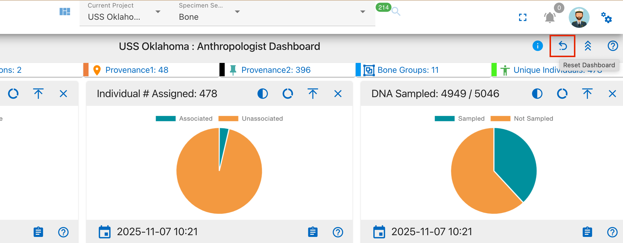
What gets reset:
- Widget positions: All widgets return to their original default positions
- Removed widgets: Any widgets you've closed/removed will reappear on the dashboard
- Custom arrangements: Your personalized drag-and-drop layout will be restored to the system default
When to use reset:
- When you want to start fresh with widget arrangement
- If you've accidentally removed important widgets and want them back quickly
- When switching between different types of analysis work that require different layouts
- To restore the dashboard after experimenting with different configurations
The reset feature provides a quick way to return to a known working state without having to manually restore each individual change.
Dashboard Widgets
Dashboards are made of many different widgets. These widgets provide visualization for the data they represent. Widgets can display Pie Charts, Line Charts, Bar Charts, Maps, etc...
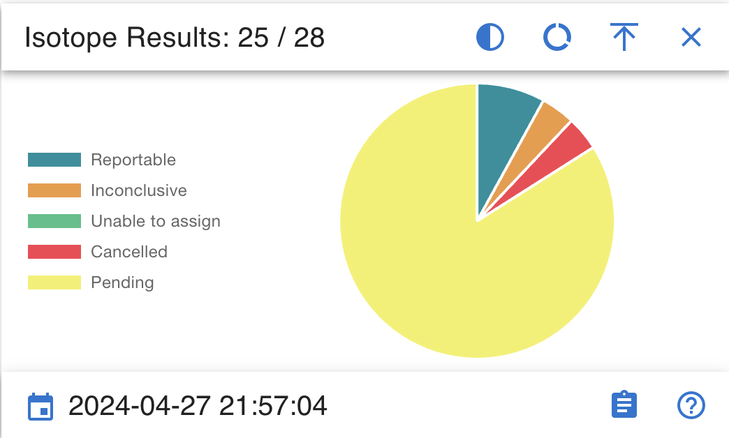
Widgets come with a handful of standard features/functions.
-
Last Updated Timestamp :- It shows the latest date when the data was updated. From the above image the last updated timestamp is shown at bottom left corner
-
Mouse Over Detail :- On hovering over the graphs present in the widgets provides information on data.

-
View Details (Drill Into The Data) :- On click of details from the widget gives all the details of the visual data represented.

-
Widget Controls :- The common widget controls present on all the widgets are
-
Collapse
-
Close

-
Help-Cora Docs

Pie Chart
The widgets that shows data in pie chart has different options to view data.
- Semi Circle:- Clicking on the semi-circle option provides a dynamic semicircle view, offering a perspective on data representation.


- Full Circle:- Clicking on the full-circle option provides a dynamic full circle view, offering a perspective on data representation.


- Show Donut:- Clicking on Donut option provides a dynamic donut view of data representation.


- Show Pie:- Clicking on Pie option provides a dynamic Pie view of data representation.


Bar Graph & Stacked Bar Graph
The widgets for bar graph has a toggle switch.
The toggle switch has 2 options:
- Show all
- Show MNI Data
If the toggle switch is deactivated, bar graph/stacked bar graph would show data for all.


If the toggle switch is activated, bar graph/stacked bar graph would show data related to MNI Only

Line Graph
The widgets that shows data in Line graph has different options to view data.
Line graph has below widget controls:
- Line Step
- Days
- Point Style
Line Step
Line step is a dropdown which shows 4 options to select from

The view of data in line graph changes depending on the Line step chosen. Below image shows data for line step selected as "before".

Days
Days is a dropdown which shows 4 options to select from

The view of data in line graph changes depending on the days selected. If the days selected is 180 or 1 year then the line graph will show a lot of data compared to days selected as 30 or 90. Below image shows data for days selected as "180 days".

Point Style
Point style is also a dropdown which shows 4 options to select from

The view of data in line graph changes depending on the point style chosen. Below image shows data when point style selected is "Triangle".

Project Dashboard
Project Manager Dashboard
The Project Manager Dashboard serves as a high level view of both summary and aggregated project data. The dashboard is comprised of widgets, which are individual visual representations of data. Examples of those widgets include:
- Skeletal Elements Associated To Individual
- DNA Sample Information
- Mito sequence Information
- Inventory Process
Those widgets can be added and removed via the widget selector.

The data in the dashboard is represented in 4 different formats:
- Pie Chart
- Bar Graph
- Stacked Bar Graph
- Line Graph
On Click of details from widgets project dashboard will be visible. It provides a detailed view of visualization and the data.
Pie Chart
Data can be visualized in different ways by widget selector for pie chart.
The data in the widgets will be seen as shown below
Clicking on the show donut option provides a dynamic semicircle view, offering a perspective on data representation.
Clicking on show pie provides a dynamic pie view, offering a perspective on data representation.
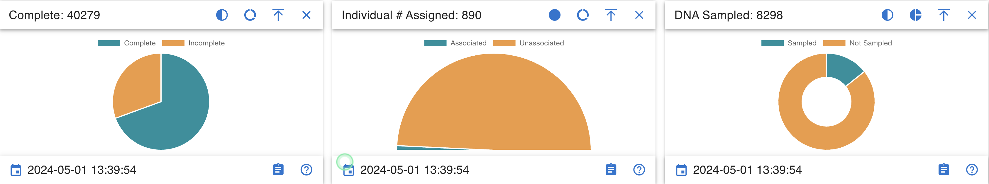
On Click of details present on widgets, provides a detailed view of the visualization along with column details.

Below are the fields that are visible:
- Key
- Bone
- Side
- Bone Group
- Individual Number
- DNA Sample Number
- Mito Sequence Number
- Associations
- Pathology
- Methods
- Measured
- Complete
- Isotope Sampled
- Clavicle Triage
- CT Scanned
- Xray Scanned
- Inventoried
- Reviewed
- Inventoried By
Bar Graph
Bar Graph helps provide comparisons between discrete categories or groups.
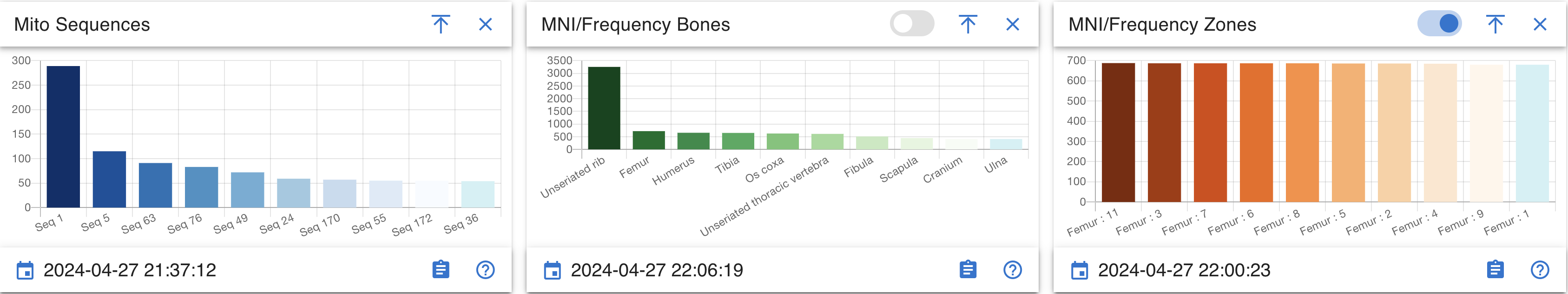
On Click of details present on widgets, provides a detailed view of the visualization along with column details.

Below are the fields that are visible:
- Mito Sequence Number
- Total
These fields will vary depending on type of module selected
Stacked Bar graph
Stacked bar graph is divided into segments or "stacks" to represent different categories or subgroups within a single category.
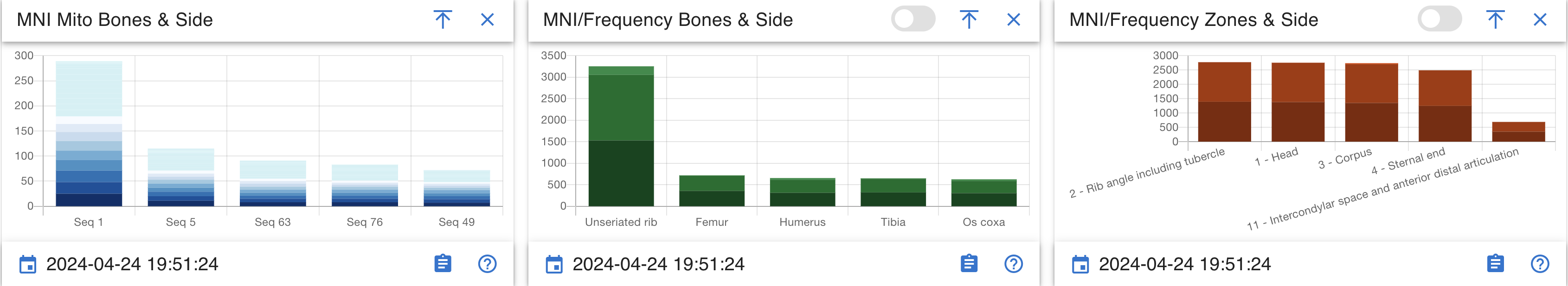
On Click of details present on widgets, provides a detailed view of the visualization along with column details.

Below are the fields that are visible:
- bone
- side
- Total
These fields will vary depending on type of module selected
Line graph
Line graph helps visualize data trends over time or across different data categories.
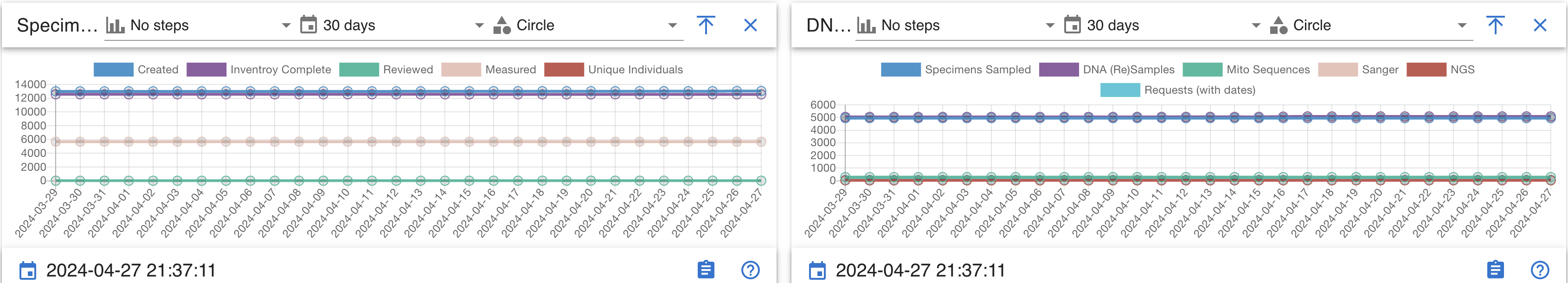
Line graph widget contains the following:
- Line step
- Days
- Point Style
Widget Details
Below is a detailed description of each widget included in the Project Dashboard, their purpose, and interaction capabilities.
Complete
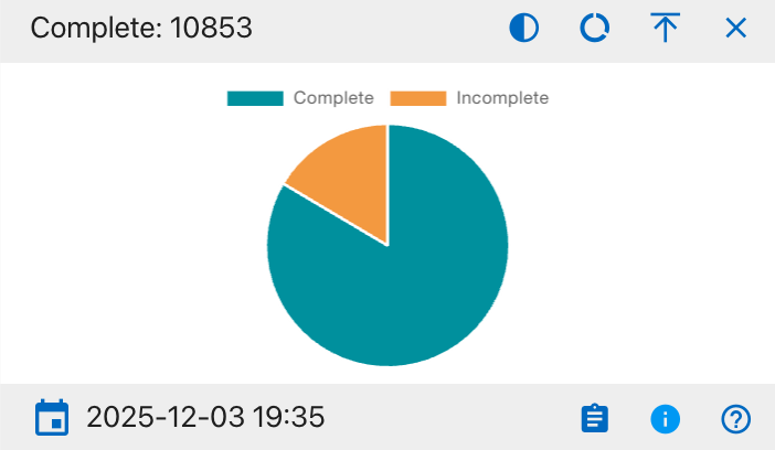
The details shown include:
- Complete
- Incomplete
This widget provides a visual breakdown of record completion status across all projects on the Project Dashboard. The pie chart displays the proportion of records that are complete versus incomplete, helping users quickly assess overall progress. Users can hover over each segment to view the exact counts and click to export the supporting table to Excel or PDF. Column visibility options are available in the integrated data table beneath the chart.
Individual Assigned
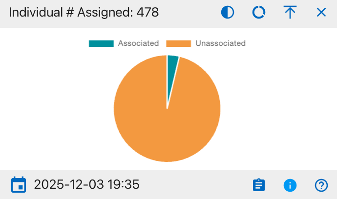
The details shown include:
- Associated
- Unassociated
This widget provides a visual breakdown of how many individual records are currently associated versus unassociated on the Project Dashboard. The pie chart displays the proportion of individuals in each category, helping users quickly see whether most individuals have been properly linked to projects. Users can hover over each segment to view the exact counts and click to export the supporting table to Excel or PDF. Column visibility options are available in the integrated data table beneath the chart.
DNA Sampled

The details shown include:
- Sampled
- Not Sampled
This widget provides a visual breakdown of DNA sampling status across all relevant records on the Project Dashboard. The pie chart displays the proportion of records that have been sampled versus not sampled, helping users quickly assess overall sampling coverage. Users can hover over each segment to view the exact counts and click to export the supporting table to Excel or PDF. Column visibility options are available in the integrated data table beneath the chart.
DNA Mito Results

The details shown include:
- Reportable
- Inconclusive
- Unable to assign
- Cancelled
- No Results
- Pending
This widget provides a visual breakdown of mitochondrial DNA (Mito) test results across all relevant records on the Project Dashboard. The pie chart displays the proportion of records in each result category, helping users quickly understand overall identification outcomes and remaining work. Users can hover over each segment to view the exact counts and click to export the supporting table to Excel or PDF. Column visibility options are available in the integrated data table beneath the chart.
DNA YSTR Results
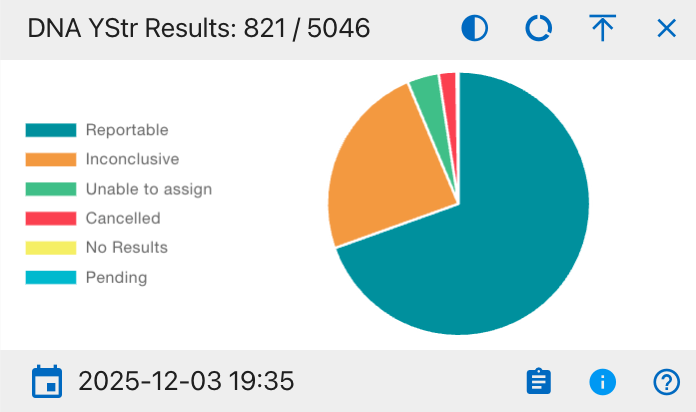
The details shown include:
- Reportable
- Inconclusive
- Unable to assign
- Cancelled
- No Results
- Pending
This widget provides a visual breakdown of YStr DNA test results across all relevant records on the Project Dashboard. The pie chart displays the proportion of records in each result category, helping users quickly understand overall YStr testing outcomes and where additional work may be required. Users can hover over each segment to view the exact counts and click to export the supporting table to Excel or PDF. Column visibility options are available in the integrated data table beneath the chart.
DNA AUSTR Results
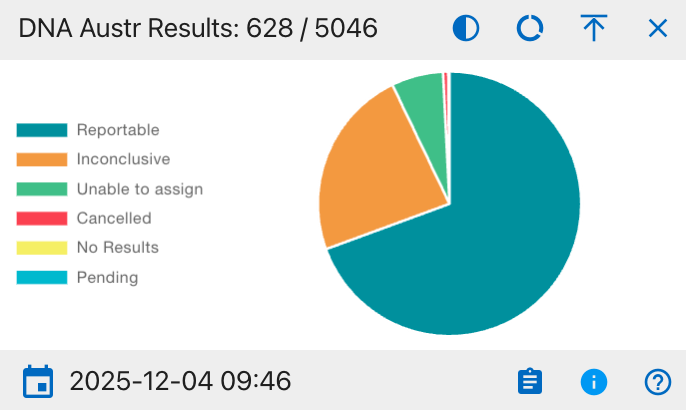
The details shown include:
- Reportable
- Inconclusive
- Unable to assign
- Cancelled
- No Results
- Pending
This widget provides a visual breakdown of AUSTR DNA test results across all relevant records on the Project Dashboard. The pie chart displays the proportion of records in each result category, helping users quickly understand overall AUSTR testing outcomes and where additional follow-up may be required. Users can hover over each segment to view the exact counts and click to export the supporting table to Excel or PDF. Column visibility options are available in the integrated data table beneath the chart.
Measured
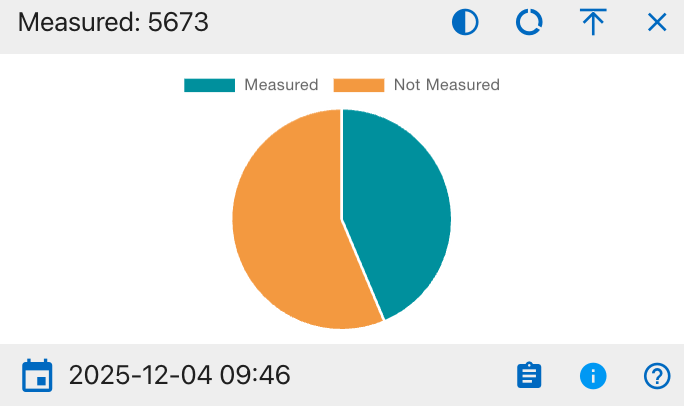
The details shown include:
- Measured
- Not Measured
This widget provides a visual breakdown of measurement status across all relevant records on the Project Dashboard. The pie chart displays the proportion of records that have been measured versus those that have not, helping users quickly assess coverage of required measurements. Users can hover over each segment to view the exact counts and click to export the supporting table to Excel or PDF. Column visibility options are available in the integrated data table beneath the chart.
CT Scanned
The details shown include: * Scanned * Not Scanned
This widget provides a visual breakdown of CT scanning status across all relevant records on the Project Dashboard. The pie chart displays the proportion of records that have undergone CT scanning versus those that have not, helping users quickly gauge imaging coverage. Users can hover over each segment to view the exact counts and click to export the supporting table to Excel or PDF. Column visibility options are available in the integrated data table beneath the chart.
XRAY Scanned
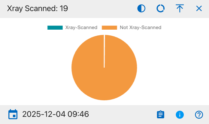
The details shown include:
- Xray-Scanned
- Not Xray-Scanned
This widget provides a visual breakdown of X-ray scanning status across all relevant records on the Project Dashboard. The pie chart displays the proportion of records that have been X-ray scanned versus those that have not, helping users quickly assess imaging coverage. Users can hover over each segment to view the exact counts and click to export the supporting table to Excel or PDF. Column visibility options are available in the integrated data table beneath the chart.
Clavicle Triage
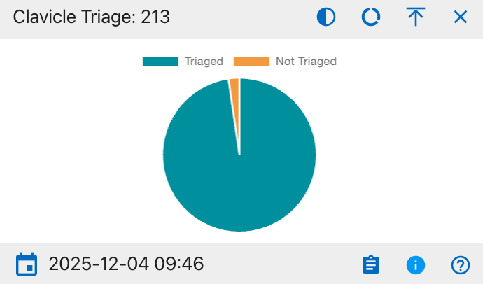
The details shown include:
- Triaged
- Not Triaged
This widget provides a visual breakdown of clavicle triage status across all relevant records on the Project Dashboard. The pie chart displays the proportion of records that have been triaged versus those that have not, helping users quickly assess progress on clavicle evaluations and identify remaining cases needing review. Users can hover over each segment to view the exact counts and click to export the supporting table to Excel or PDF. Column visibility options are available in the integrated data table beneath the chart.
Isotope Sampled

The details shown include:
- Sampled
- Not Sampled
This widget provides a visual breakdown of isotope sampling status across all relevant records on the Project Dashboard. The pie chart displays the proportion of records that have isotope samples collected versus those that have not, helping users quickly identify the current level of isotope sampling coverage and remaining cases needing sampling. Users can hover over each segment to view the exact counts and click to export the supporting table to Excel or PDF. Column visibility options are available in the integrated data table beneath the chart.
Remains Status
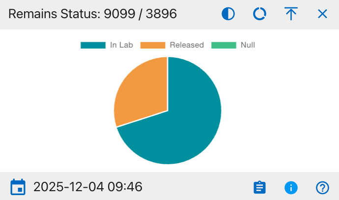
The details shown include:
- In Lab
- Released
- Null
This widget provides a visual breakdown of the current status of remains across all relevant records on the Project Dashboard. The pie chart displays the proportion of remains that are still in the lab, those that have been released, and those with a null or unspecified status, helping users quickly understand overall case disposition and remaining lab workload. Users can hover over each segment to view the exact counts and click to export the supporting table to Excel or PDF. Column visibility options are available in the integrated data table beneath the chart.
Inventoried
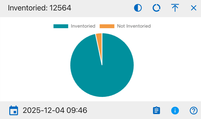
The details shown include:
- Inventoried
- Not Inventoried
This widget provides a visual breakdown of inventory status across all relevant records on the Project Dashboard. The pie chart displays the proportion of records that have been fully inventoried versus those that have not, helping users quickly assess inventory completion and identify any remaining items requiring cataloging. Users can hover over each segment to view the exact counts and click to export the supporting table to Excel or PDF. Column visibility options are available in the integrated data table beneath the chart.
Reviewed
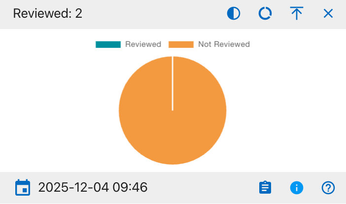
The details shown include:
- Reviewed
- Not Reviewed
This widget provides a visual breakdown of review status across all relevant records on the Project Dashboard. The pie chart displays the proportion of records that have been formally reviewed versus those still awaiting review, helping users quickly see overall QA progress and identify items that need attention. Users can hover over each segment to view the exact counts and click to export the supporting table to Excel or PDF. Column visibility options are available in the integrated data table beneath the chart.
Mito Sequence Number
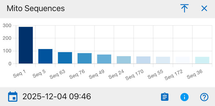
This widget displays the distribution of mitochondrial DNA (mito) sequence groups across all relevant records on the Project Dashboard. Each bar represents a different sequence group (for example, Seq 1, Seq 5, Seq 63), and the bar height shows how many records fall into that sequence, allowing users to see which mito sequences are most common and to spot patterns that may inform comparative or kinship analysis. Users can hover over each segment to view the exact counts and click to export the supporting table to Excel or PDF. Column visibility options are available in the integrated data table beneath the chart.
MNI Bones
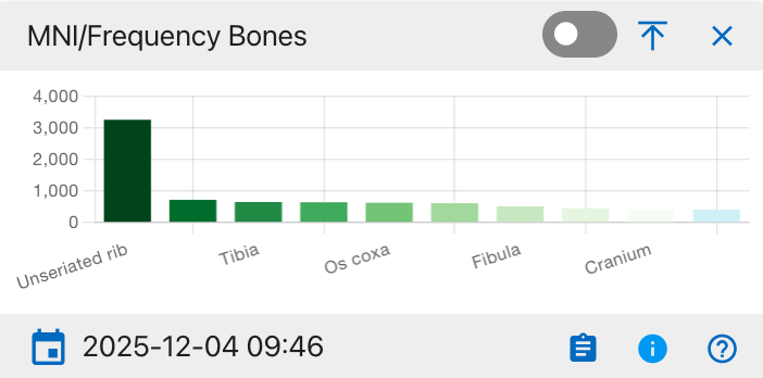
This widget shows the distribution of bones by either minimum number of individuals (MNI) or element frequency across all records on the Project Dashboard. Each bar represents a specific skeletal element (for example, unseriated ribs, tibia, os coxa, fibula, cranium), and the bar height indicates how many occurrences of that element are recorded, helping users see which bones are most frequently represented in the assemblage and guiding sampling or analysis priorities. Users can hover over each segment to view the exact counts and click to export the supporting table to Excel or PDF. Column visibility options are available in the integrated data table beneath the chart.
MNI Zones
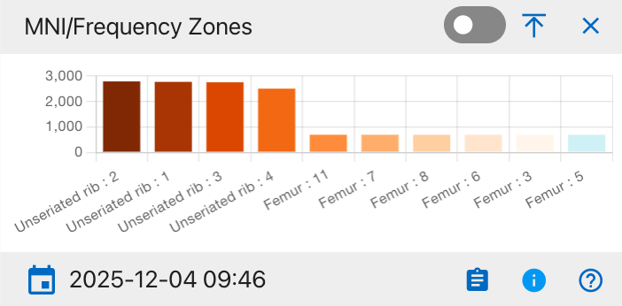
This widget shows the distribution of anatomical zones (for example, specific rib zones and femur zones) by minimum number of individuals (MNI) or occurrence frequency across all records on the Project Dashboard. Each bar represents a particular zone label (such as unseriated rib zones 1–4 or numbered femur zones), and the bar height indicates how many times that zone is present, helping users pinpoint which skeletal zones are most commonly observed and prioritize detailed recording or analysis. Users can hover over each segment to view the exact counts and click to export the supporting table to Excel or PDF. Column visibility options are available in the integrated data table beneath the chart.
MNI Mito Bones Side
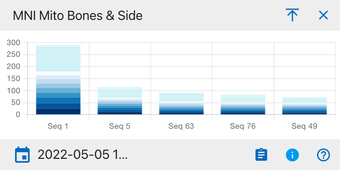
This widget uses a stacked bar chart to display, for each mitochondrial sequence group (for example, Seq 1, Seq 5, Seq 63), the minimum number of individuals (MNI) broken down by skeletal element and body side. Each vertical bar represents one sequence group, and the colored segments stacked within that bar correspond to different bones and left/right sides, so the total bar height shows the overall MNI for that sequence while the segment heights show how much each element and side contributes to that total. Users can hover over each segment to view the exact counts and click to export the supporting table to Excel or PDF. Column visibility options are available in the integrated data table beneath the chart.
MNI Bones Side
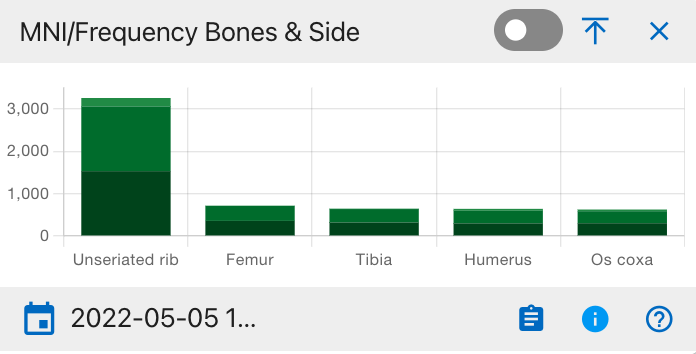
This widget shows, for each major skeletal element (for example, unseriated rib, femur, tibia, humerus, os coxa), the count or minimum number of individuals (MNI) broken down by body side. Each vertical bar represents one bone, and the stacked segments within that bar correspond to left and right sides (and, if used, midline or unspecified), so the total bar height reflects the overall frequency or MNI for that element while the segment heights show how much each side contributes. Users can hover over each segment to view the exact counts and click to export the supporting table to Excel or PDF. Column visibility options are available in the integrated data table beneath the chart.
MNI Zones Side
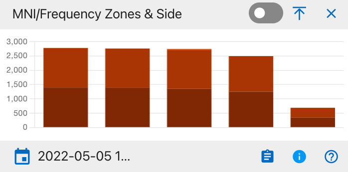
This widget shows, for each defined anatomical zone group, the count or minimum number of individuals (MNI) broken down by body side. Each vertical stacked bar represents one zone group, and the darker and lighter segments within the bar correspond to left and right (and, where applicable, midline or unspecified) sides, so the total bar height reflects the overall frequency or MNI for that zone while the segment heights show the contribution of each side. Users can hover over each segment to view the exact counts and click to export the supporting table to Excel or PDF. Column visibility options are available in the integrated data table beneath the chart.
MNI Bone Groups
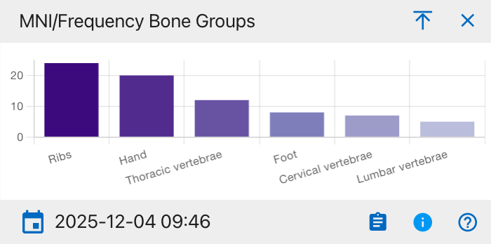
This widget shows the count or minimum number of individuals (MNI) summarized by higher-level skeletal groups, such as ribs, hand, thoracic vertebrae, foot, cervical vertebrae, and lumbar vertebrae. Each bar represents one bone group, and its height indicates how many occurrences or individuals are represented in that group, helping users quickly see which skeletal regions are most prevalent in the assemblage. Users can hover over each segment to view the exact counts and click to export the supporting table to Excel or PDF. Column visibility options are available in the integrated data table beneath the chart.
MNI Bone Groups and Side
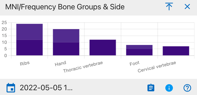
This widget shows the count or minimum number of individuals (MNI) summarized by higher-level skeletal groups, such as ribs, hand, thoracic vertebrae, foot, cervical vertebrae, and lumbar vertebrae. Each bar represents one bone group, and its height indicates how many occurrences or individuals are represented in that group, helping users quickly see which skeletal regions are most prevalent in the assemblage. Users can hover over each segment to view the exact counts and click to export the supporting table to Excel or PDF. Column visibility options are available in the integrated data table beneath the chart.
Specimens
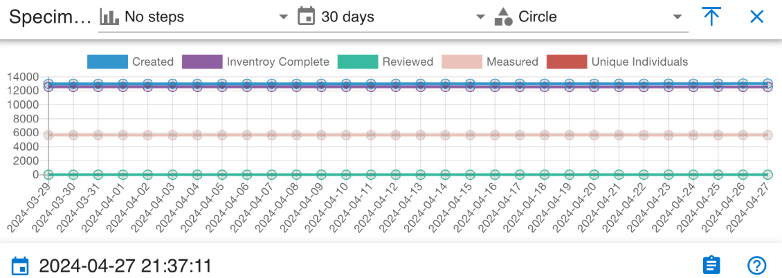
This widget is a time‑series line chart that tracks specimen workflow activity over the selected 30‑day period. Each line represents a different status count-Created, Inventory Complete, Reviewed, Measured, and Unique Individuals so users can see how many specimens are in each state on each date and quickly assess whether work volume or completion is changing over time. Users can hover over each segment to view the exact counts and click to export the supporting table to Excel or PDF. Column visibility options are available in the integrated data table beneath the chart.
DNAS
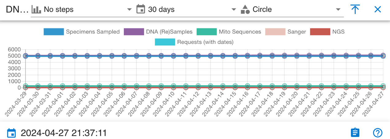
This widget is a time‑series line chart that tracks key DNA‑related workflow metrics over the selected 30‑day period. Each line represents a different metric—Specimens Sampled, DNA (Re)Samples, Mito Sequences, Sanger, NGS, and Requests (with dates),so users can see how many items fall into each category on each date and monitor trends or stability in DNA sampling, sequencing, and request activity across the month. Users can hover over each segment to view the exact counts and click to export the supporting table to Excel or PDF. Column visibility options are available in the integrated data table beneath the chart.
Cabanatuan Project Manager Dashboard
The dashboard displays an interactive cemetery map with numbered grave plots. Selecting a highlighted grave will update the panels and widgets to show information for the related burials and accessions.
Navigation
From the top navigation, select Project Dashboard to open the main interface for the Cabanatuan POW Camp.
We can see the dashboard for Cabanatuan
Cabanatuan Cemetery Map
The Cabanatuan dashboard map shows a simple layout of the POW cemetery, with each grave drawn as a numbered rectangle so you can quickly see where plots are located. Highlighted plots show the graves that are currently in view for the project, and clicking one of these plots focuses the dashboard on that grave and its related accessions, helping you connect the cemetery layout to the underlying case records.
Filters
Use the filters above the map to refine which graves and records are shown. You can filter by:
- Accessions
- Common Graves / Provenance
- Dates From
- Dates To
Click Apply to activate the filters or Reset to clear them and return to the full Cabanatuan view.
Widgets
Widgets below the map summarize key information about the Cabanatuan project.
The main widget groups include:
- Workflow Status – Complete, Individuals Assigned, Inventoried, Reviewed, Measured, X‑ray Scanned, CT Scanned, Isotope Sampled, Clavicle Triage, Remains Status.
- DNA Sampling and Results – DNA Sampled, DNA Mito Results, DNA YSTR Results, DNA AUSTR Results, Mito Sequences.
- Skeletal Representation (MNI/Frequency) – Bones, Bones & Side, Zones, Zones & Side, Bone Groups.
- Activity Over Time – 30‑day lines for specimen steps (Created, Inventory Complete, Reviewed, Measured, Unique Individuals) and for DNA steps (Specimens Sampled, DNA (Re)Samples, Mito Sequences, Sanger, NGS, Requests).
DNA Dashboard
The DNA Dashboard provides a centralized view of DNA testing progress and results across the organization. It summarizes key performance indicators (KPIs) from mitochondrial (Mito), autosomal (AuSTR), and Y-STR analyses, allowing administrators and analysts to monitor laboratory efficiency, report generation, and sequencing outcomes.
Navigation
From the main sidebar, click on DNA Dashboard under the DNA section. The interface will display a set of visual KPI widgets and line chart representing summarized data for all DNA records.

This dashboard integrates live data from the DNA module - including fields such as sample methods, received dates, sequencing counts, and report statuses.
Widget Features
Each widget in the DNA Dashboard comes with standard features similar to other dashboards:
- Last Updated Timestamp - Shows when the DNA data was last updated

- Mouse Over Detail - Hover over charts for detailed DNA statistics
- View Details (Drill Into The Data) - Click for detailed DNA sample information
-
Widget Controls:
-
Collapse - Minimize the widget to save space while keeping it accessible
- Close - Remove the widget from the dashboard view
- Help-Cora Docs - Access detailed documentation and usage guides
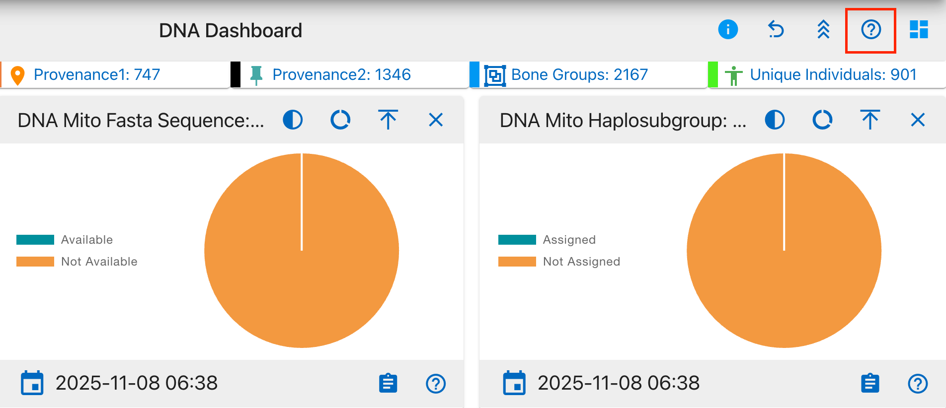
Pie Chart Visualization
Most DNA metrics are displayed as pie charts showing:
- Clear color coding for different categories
- Percentage distribution
- Interactive tooltips on hover
- Detailed legends
Chart Visualization Types
The DNA Dashboard offers three different chart styles to effectively visualize data distributions:
1 Full Pie Chart
The traditional 360-degree circular chart that shows the complete proportion of all components. Best used for:
- Displaying part-to-whole relationships
- Comparing multiple categories
- Showing percentage distributions
- Visualizing complete data sets with clear segment differences
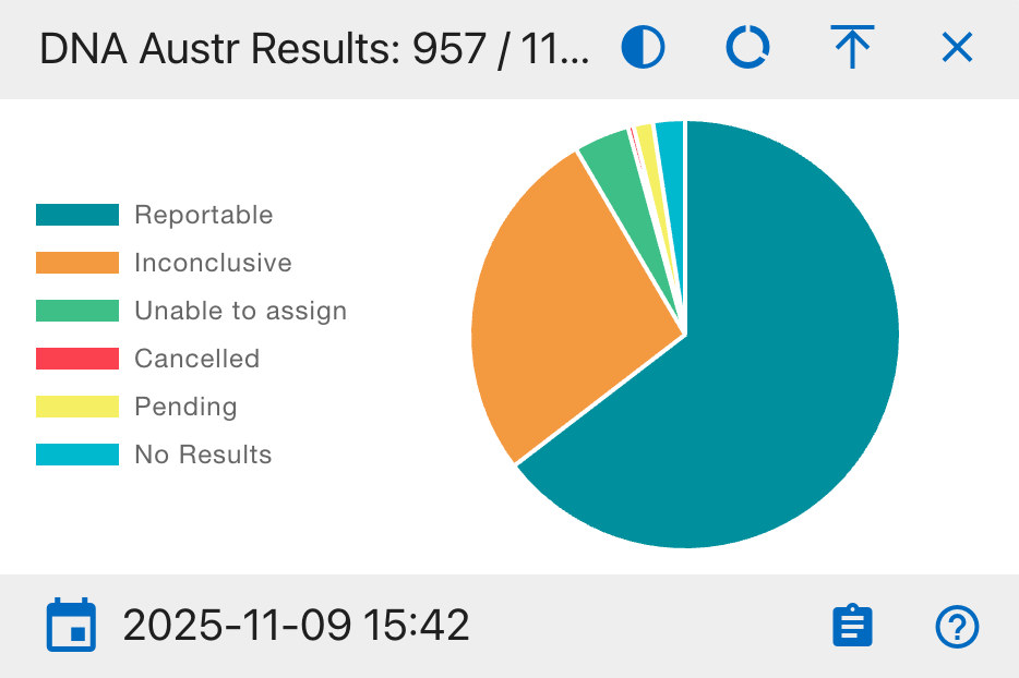
2 Half Pie Chart
A 180-degree semicircular visualization that offers a more compact view. Ideal for:
- Space-efficient data presentation
- Binary comparisons (e.g., Completed vs. Pending)
- Dashboard layouts where vertical space is limited
- Emphasizing simple proportional relationships
3 Donut Chart
A circular chart with a hollow center that emphasizes individual segments. Particularly effective for:
- Focusing on individual segment values
- Displaying additional information in the center
- Multi-layer data presentation
- Emphasizing the relationship between parts while maintaining visual distinction
Each chart type maintains interactive features such as hover tooltips, click-through capabilities, and real-time updates.
General Notes
- Each chart segment is clickable and supports drilldown exploration.
- Hovering over segments shows precise counts and percentages.
- Widgets update automatically when DNA data changes or processing is completed.
- Timestamps indicate the last data refresh.
- All widgets maintain consistent color coding across the dashboard.
- Data can be exported in multiple formats (CSV, PDF, Print).
- Filters allow focusing on specific date ranges or sample types.
KPI Widgets
KPIs in the DNA Dashboard are interactive visual elements that provide real-time insights into critical DNA testing metrics.
The widgets are categorized into three main DNA testing areas:
- Mitochondrial DNA (Mito) - Maternal lineage analysis
- Autosomal DNA (AuSTR) - Genetic inheritance patterns
- Y-chromosome DNA (Y-STR) - Paternal lineage tracking
Below is a comprehensive description of each widget available in the DNA Dashboard, including their purpose, data interpretation guidelines, and practical applications in DNA analysis workflows.
DNA Mito Results
A comprehensive pie chart showing the distribution of mitochondrial DNA testing results
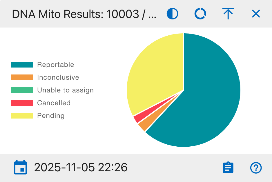
Pie Chart Segments:
- Reportable
- Inconclusive
- Unable to assign
- Cancelled
- Pending
This widget helps analysts track testing progress and identify potential bottlenecks in the DNA analysis workflow.
DNA Mito Methods
A comprehensive view of DNA sequencing methods used in the laboratory
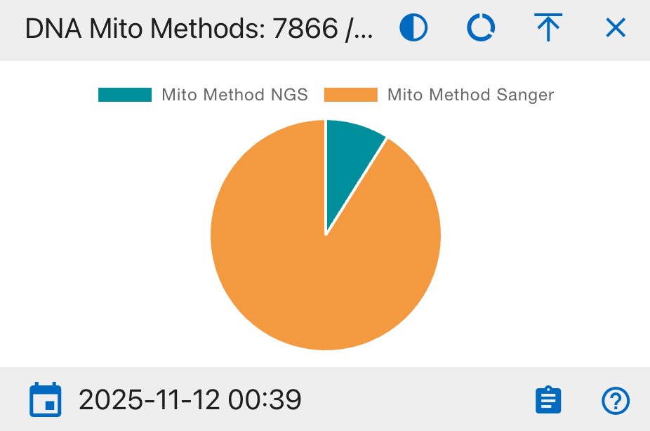
Pie Chart Segments:
- Mito Method NGS
- Mito Method Sanger
This widget helps track the adoption of different sequencing technologies and monitor resource allocation across methods.
DNA Mito Counts
A statistical overview of DNA sample matching status
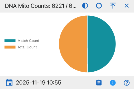
Pie Chart Segments:
- Match Count
- Total Count
This widget provides insights into the success rate of DNA matching processes and helps evaluate overall testing efficiency.
DNA Mito Dates
A timeline analysis of DNA sample processing status
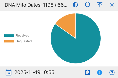
Pie Chart Segments:
- Received
- Requested
This widget helps monitor laboratory workflow efficiency and identify potential processing backlogs.
DNA Mito Sequence
A detailed breakdown of DNA sequence categorization
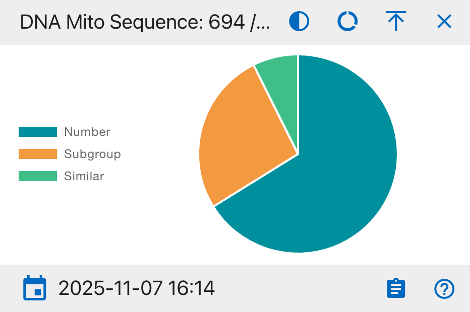
Pie Chart Segments:
- Number
- Subgroup
- Similar
This widget facilitates the identification of sequence patterns and potential familial connections in the database.
DNA Mito Haplogroup
A tracking system for ancestral lineage classification
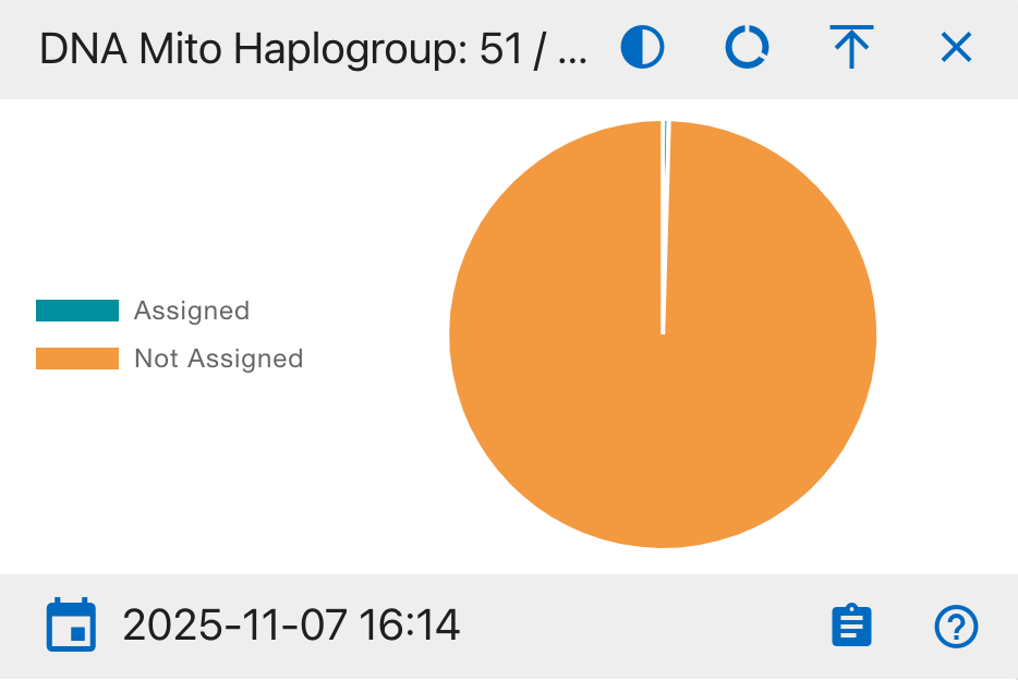
Pie Chart Segments:
- Assigned
- Not Assigned
This widget monitors the progress of maternal lineage classification and geographical origin determination.
DNA Mito Confirmed Regions
A quality assurance overview of DNA region verification
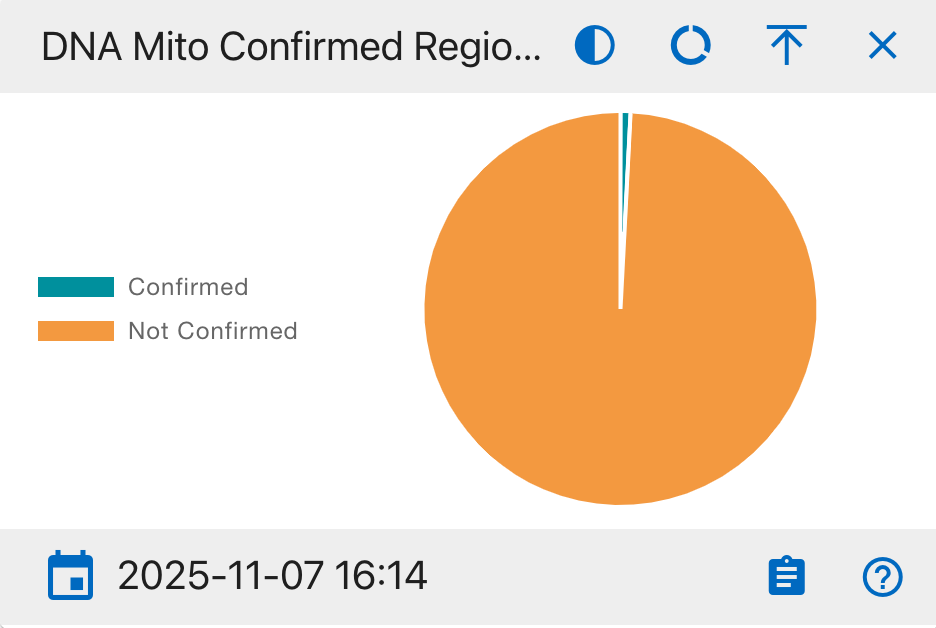
Pie Chart Segments:
- Confirmed
- Not Confirmed
This widget is essential for quality control processes and helps ensure the accuracy of DNA analysis results. It tracks the verification status of analyzed DNA regions.
DNA Mito Base Pairs
A detailed view of base pair sequencing completion
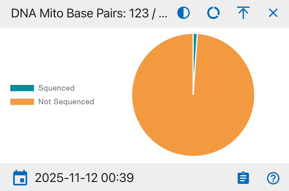
Pie Chart Segments:
- Sequenced
- Not Sequenced
This widget monitors the granular progress of DNA sequencing at the base pair level, crucial for ensuring complete genetic analysis coverage.
DNA Mito Polymorphisms
An analysis of genetic variation patterns in mitochondrial DNA
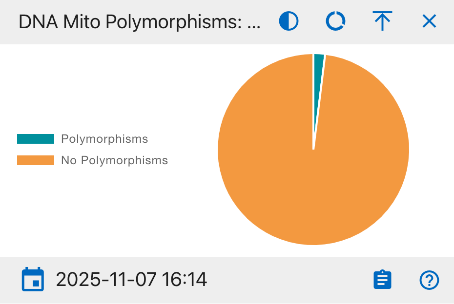
Pie Chart Segments:
- Polymorphisms
- No Polymorphisms
This widget helps identify genetic diversity by tracking the presence of DNA sequence variations, essential for population genetics studies and individual identification.
DNA Mito Fasta Sequence
A tracker for standardized DNA sequence file availability
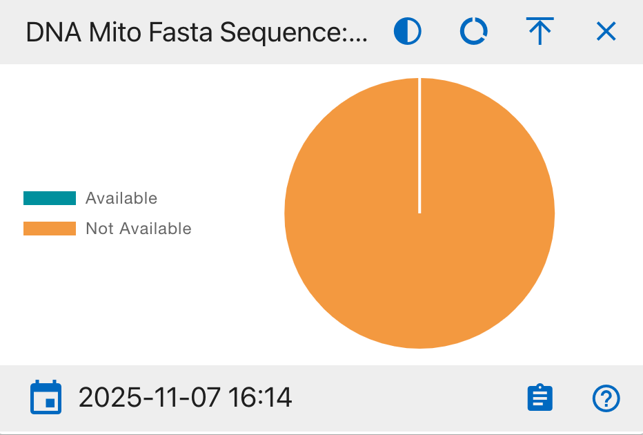
Pie Chart Segments:
- Available
- Not Available
This widget monitors the availability of DNA sequences in the standardized FASTA format, which is essential for bioinformatics analysis and data sharing between systems.
DNA Mito Haplosubgroup
A detailed breakdown of mitochondrial DNA subgroup classifications

Pie Chart Segments:
- Assigned
- Not Assigned
This widget tracks the detailed classification of maternal lineages into specific subgroups, providing finer granularity for population genetics and ancestry studies.
DNA Mito Loci
A status overview of genetic marker analysis progress
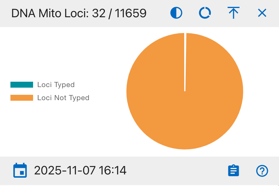
Pie Chart Segments:
- Loci Typed
- Loci Not Typed
This widget monitors the progress of genetic marker typing, essential for comprehensive DNA profiling and accurate genetic comparisons.
DNA Mito MCC Dates
A tracking system for Multi-Copy Control review status
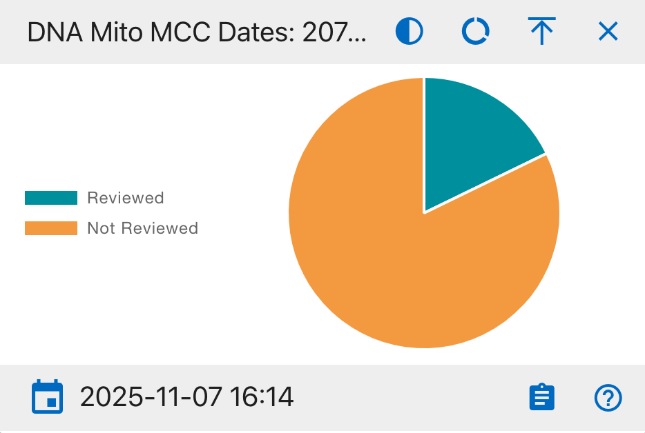
Pie Chart Segments:
- Reviewed
- Not Reviewed
This widget monitors the progress of Multi-Copy Control (MCC) reviews, which are critical for quality assurance and validation of DNA analysis results.
DNA Sample Condition
A comprehensive tracker for physical DNA sample status
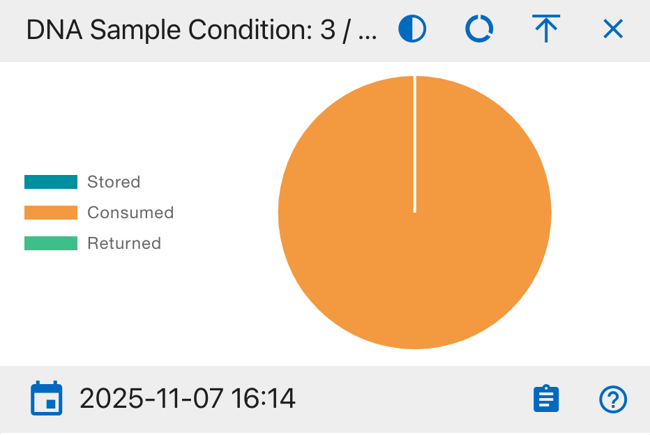
Pie Chart Segments:
- Stored
- Consumed
- Returned
This widget provides crucial inventory management information, tracking the physical status and location of all DNA samples throughout their lifecycle.
DNA Resampled
A tracking system for DNA sample retesting status
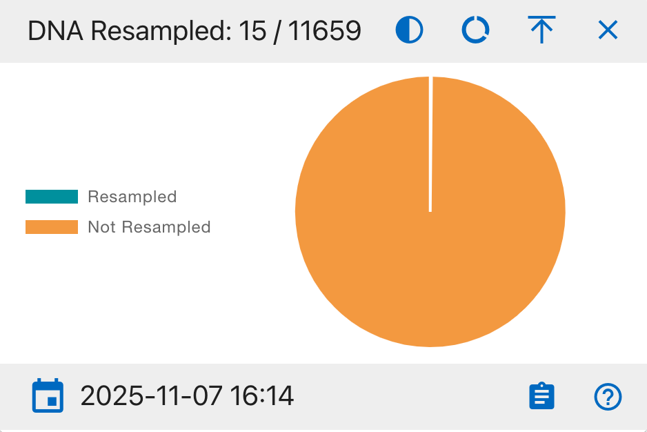
Pie Chart Segments:
- Resampled
- Not Resampled
This widget monitors the frequency of DNA resampling, helping identify quality control patterns and potential testing issues.
DNA BTB Dates
A timeline comparison of DNA testing requests and results
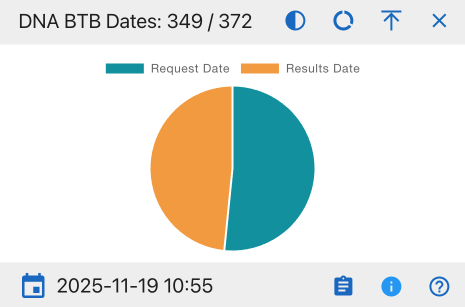
Pie Chart Segments:
- Request Date
- Results Date
This widget helps track the turnaround time between DNA test requests and result availability, supporting workflow optimization.
DNA Austr Methods
A comprehensive overview of austr DNA testing method assignments
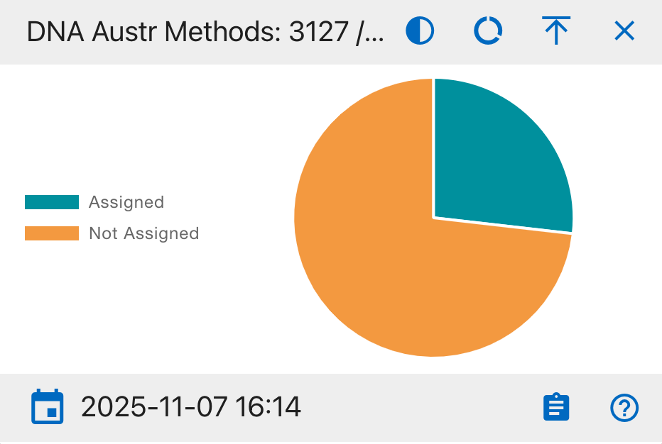
Pie Chart Segments:
- Assigned
- Not Assigned
This widget helps track the status of method assignments for austr DNA testing, ensuring proper testing protocols are followed and identifying samples that need method designation.
DNA Austr Results
A comprehensive overview of austr DNA testing outcomes
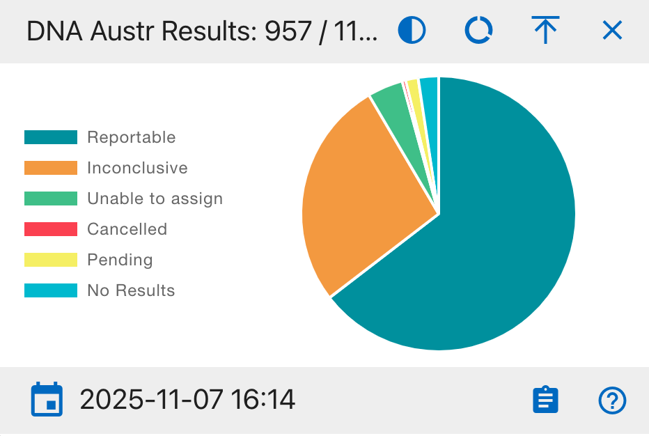
Pie Chart Segments:
- Reportable
- Inconclusive
- Unable to assign
- Cancelled
- Pending
- No Results
This widget provides a complete view of austr DNA testing outcomes, helping analysts track success rates and identify potential issues in the testing process.
DNA Austr Dates
A timeline analysis of austr DNA sample processing
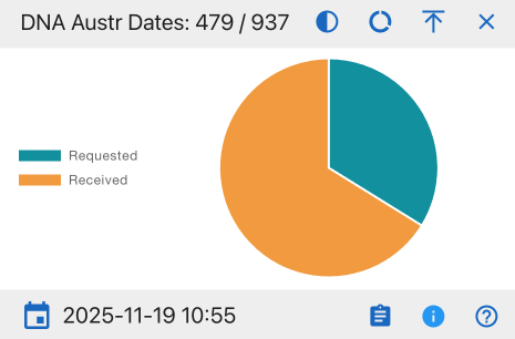
Pie Chart Segments:
- Requested
- Received
This widget monitors the flow of austr DNA samples through the laboratory system, helping identify processing bottlenecks.
DNA Austr Sequence
A categorical analysis of austr DNA sequence data
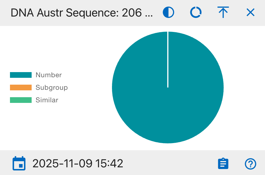
Pie Chart Segments:
- Number
- Subgroup
- Similar
This widget provides insight into the distribution and relationships of austr DNA sequences, helping identify patterns and potential matches.
DNA Austr Loci
A status overview of austr DNA marker analysis

Pie Chart Segments:
- Loci Typed
- Loci Not Typed
This widget tracks the progress of genetic marker typing for austr DNA, essential for complete DNA profiling and identification.
DNA Austr MCC Dates
A tracking system for austr DNA Multi-Copy Control review status
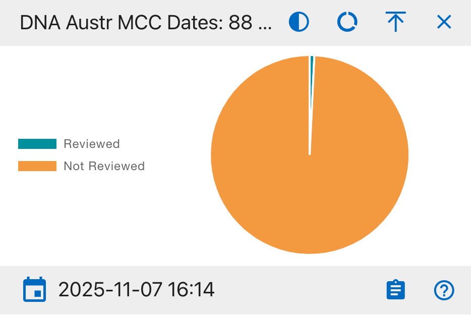
Pie Chart Segments:
- Reviewed
- Not Reviewed
This widget monitors the progress of Multi-Copy Control (MCC) reviews for autosomal DNA samples, ensuring quality control standards are met.
DNA YStr Methods
A comprehensive overview of YStr DNA testing method assignments
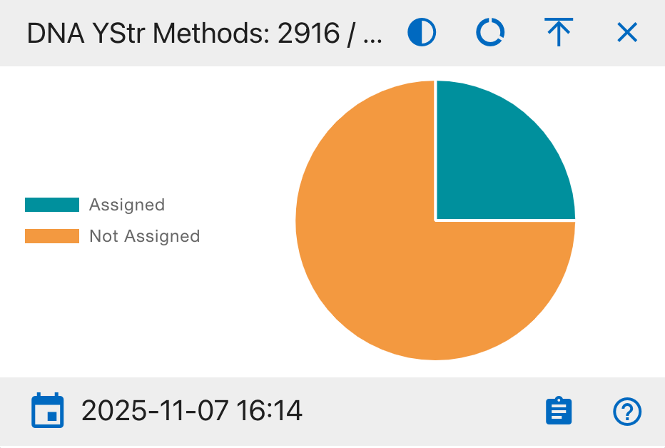
Pie Chart Segments:
- Assigned
- Not Assigned
This widget tracks the status of method assignments for YStr DNA testing, ensuring appropriate testing protocols are followed.
DNA YStr Results
A comprehensive overview of YStr DNA testing outcomes

Pie Chart Segments:
- Reportable
- Inconclusive
- Unable to assign
- Cancelled
- Pending
- No Results
This widget provides a complete view of YStr DNA testing outcomes, helping analysts track success rates and identify potential issues in the testing process.
DNA YStr Dates
A timeline analysis of YStr DNA sample processing status
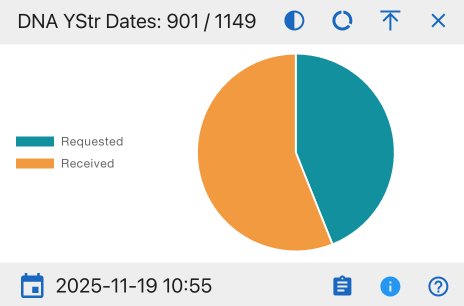
Pie Chart Segments:
- Requested
- Received
This widget helps monitor laboratory workflow efficiency and identify potential processing backlogs by tracking the number of YStr DNA samples requested versus those received.
DNA YStr Sequence
A categorical analysis of Y-STR DNA sequence data
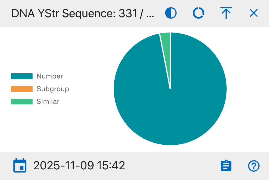
Pie Chart Segments:
- Number
- Subgroup
- Similar
This widget provides insight into the distribution and relationships of YStr DNA sequences, helping identify patterns and potential matches.
DNA YStr Loci
A status overview of Y-STR DNA genetic marker analysis

Pie Chart Segments:
- Loci Typed
- Loci Not Typed
This widget tracks the progress of genetic marker typing for YStr DNA samples, essential for complete DNA profiling and identification.
DNA YStr Counts
A statistical overview of Y-STR DNA sample matching status
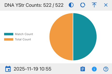
Pie Chart Segments:
- Match Count
- Total Count
This widget provides insights into the success rate of YStr DNA matching processes and helps evaluate overall testing efficiency.
DNA YStr MCC Dates
A tracking system for Y-STR DNA Multi-Copy Control review status
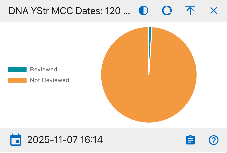
Pie Chart Segments:
- Reviewed
- Not Reviewed
This widget monitors the progress of Multi-Copy Control (MCC) reviews for YStr DNA samples, which are critical for quality assurance and validation of DNA analysis results.
DNA line Chart
The bottom section features a comprehensive DNA timeline showing multiple data series in a line graph format:
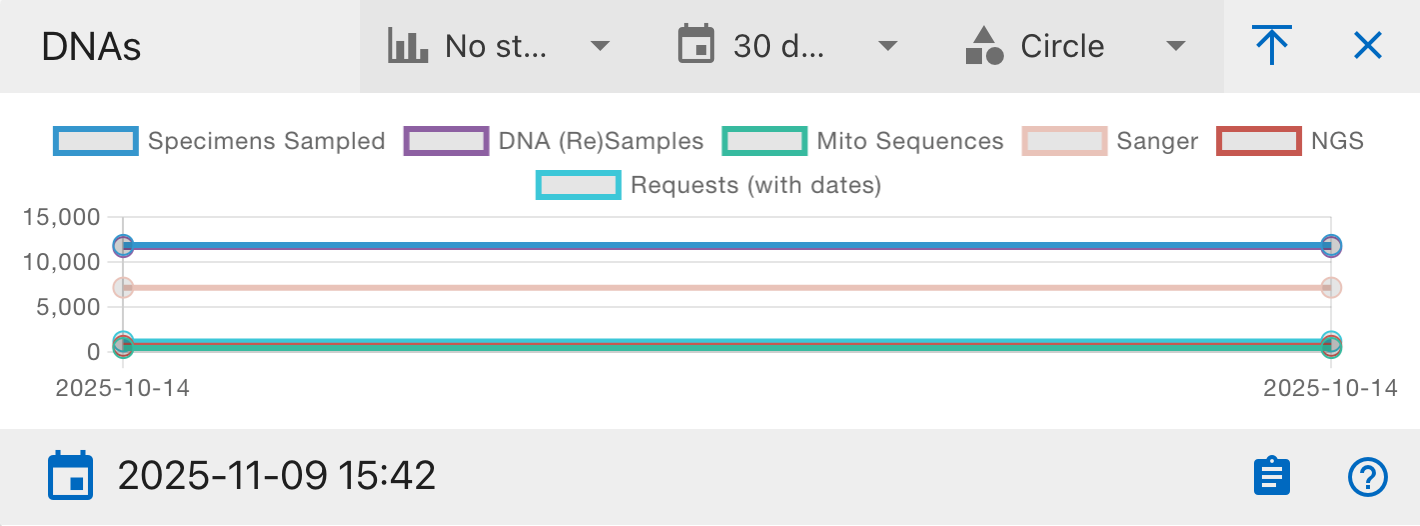
Data Series:
- Specimens Sampled
- DNA (Re)Samples
- Mito Sequences
- Sanger
- NGS
- Requests
The Y-axis shows the count (ranging from 0 to 15,000) while the X-axis shows the date range.
Graph Controls:
- No step/Step options - Toggle between continuous or stepped line visualization
- 30 days time range selector - Adjust the time window for analysis
- Circle point style option - Toggle data point markers
- Full screen toggle - Expand the graph for detailed viewing
The graph updates in real-time and shows the timestamp of the last update. This visualization helps track trends and relationships between different DNA processing stages over time.
Individual Dashboard
Warning
This page is work in progress.
The Individual dashboard provides at a glance high level charts and tables of data, statistics and charts.
Isotope Dashboard
The Isotope Dashboard provides a comprehensive visual overview of isotopic data and laboratory progress within CoRA.
It helps analysts, isotope specialists, and researchers monitor the entire workflow from demineralization and collagen extraction to isotope measurement and ratio analysis through interactive charts and analytical metrics.
Accessing the Isotope Dashboard
To open the Isotope Dashboard:
Dashboard Overview
Once the page loads, you’ll see a collection of draggable, collapsible, and interactive widgets.
Each widget represents a unique phase or analytical aspect of isotope processing from sample results to elemental isotope analyses.
The dashboard includes pie charts, donut charts, and a timeline chart that visually summarize data completeness and lab progress across projects.
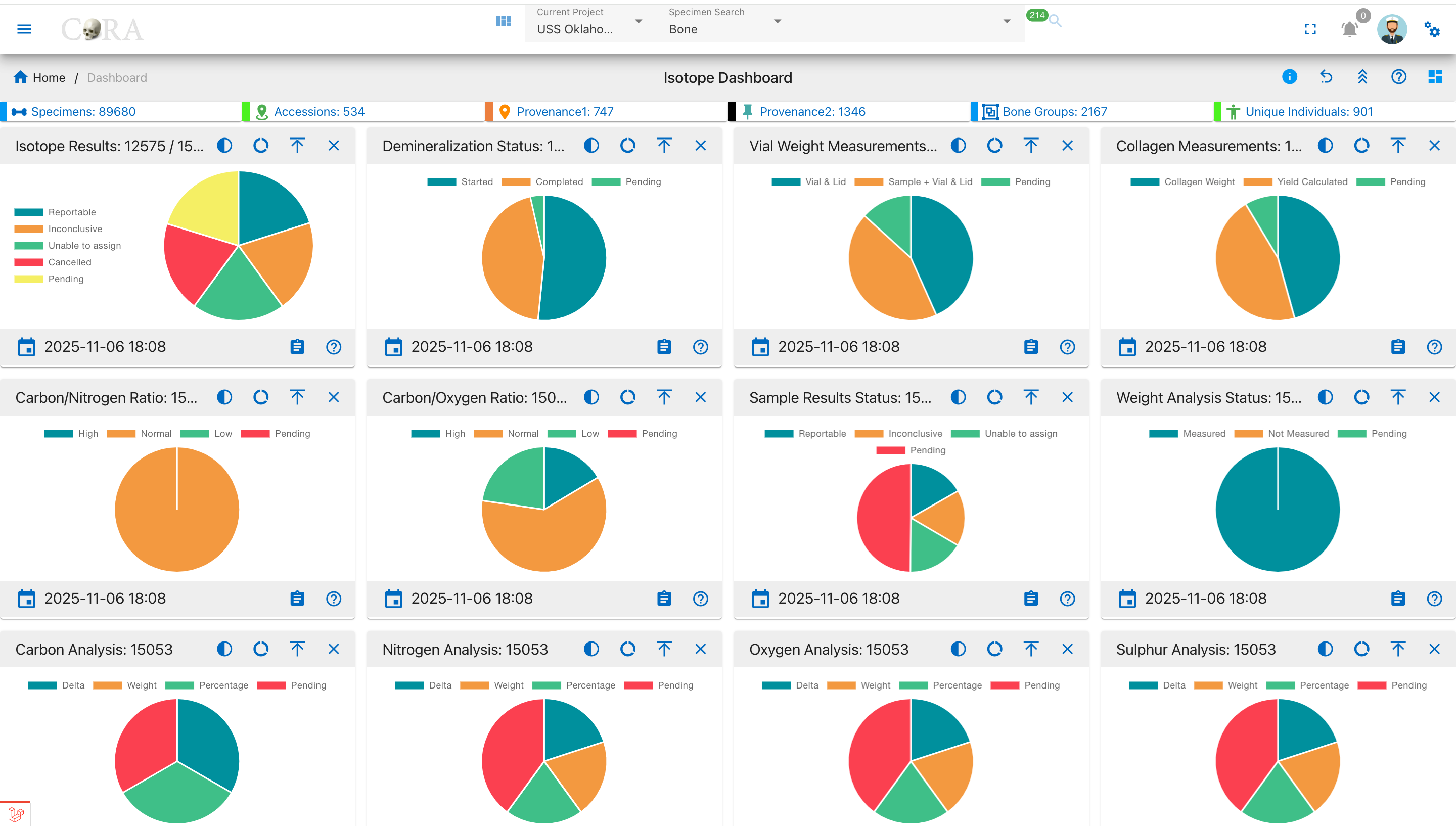
Widget Interaction
Each widget in the dashboard is fully interactive and customizable:
Collapse / Expand
- To manage all widgets at once, use the Collapse All / Expand All buttons at the top of the dashboard.
Drilldown

- Click any pie segment or chart bar to view detailed, filtered data for that specific category (e.g., Reportable Results).
Reorder Widgets
- Click and drag widgets to rearrange them on the dashboard.
- The layout is automatically saved in your browser’s localStorage, so your preferences persist between sessions.
Timestamp

- Each widget shows a timestamp (e.g., 2025-11-05 18:24) at the bottom, indicating when its data was last refreshed.
Chart Controls and Visualization Modes
Every widget contains a set of chart control icons in the top right corner.
These controls help users customize visualization, open documentation, and manage layout making interpretation of isotope data more intuitive.
Chart Control Icons
| Icon | Name | Function / Description |
|---|---|---|
| ? (Help Link) | Documentation Access | Opens the related CoRA User Documentation in a new tab. This helps users understand the scientific process behind that widget (e.g., Demineralization, Collagen Yield, or Isotope Analysis). |
| ⭘ / ◉ / ◔ | Chart Type Toggle | Switches between: - Full Pie: complete dataset view. - Half Pie: highlights progress (e.g., completed vs pending). - Donut: shows a ringed chart emphasizing proportions. |
| ⇵ (Collapse) | Toggle Visibility | Minimizes or expands the widget body while keeping its title visible. |
| × (Close) | Remove Widget | Temporarily hides the widget from the view; restoring it requires page refresh. |
Chart Visualization Types
1 Full Pie Chart
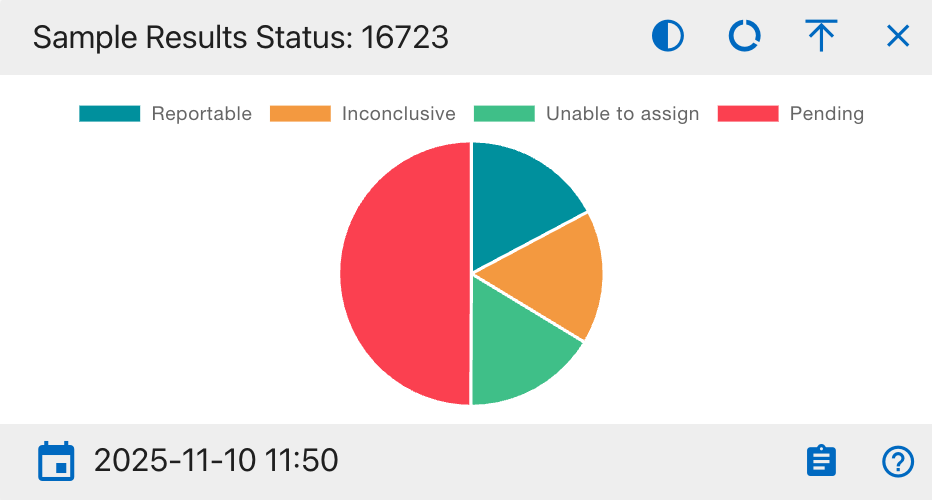
- Displays the complete dataset as a 360° circle.
- Best for viewing category distribution.
- Each color segment shows its proportional share out of the total.
Use when: You want a full snapshot of how data is distributed across categories.
2 Half Pie Chart
- Shows only the top half of the chart ideal for progress visualization (e.g., completed vs pending).
- Provides a clean comparison of workflow completion rates.
Use when: You want to monitor lab progress or readiness visually.
3 Donut Chart
- Displays the chart as a ring with a hollow center.
- The empty middle area draws attention to completed vs remaining work.
- Often used for ratio and yield comparisons.
Use when: You want to emphasize proportional completeness or compare processed vs unprocessed data.
4 “?” Help Link Integration
Each widget contains a question mark (?) icon linking directly to CoRA’s official User Documentation.
This feature connects real-time analytics to the lab procedures that generate the data.
Tips for Users
- Use Donut Mode for visual progress tracking.
- Use Half Pie Mode for workflow monitoring.
- Click ? to access the relevant CoRA docs for step by step explanations.
- Expand (⤢) and switch to Full Pie for detailed reviews.
Understanding the Dashboard Widgets
Each widget in the Isotope Dashboard visualizes a specific isotopic analysis process or metric.
All are color-coded, interactive, and linked to drilldown views for deeper exploration.
General Notes
- Each chart segment is clickable and supports drilldown exploration.
- Hovering over segments shows precise counts and percentages.
- Widgets update automatically when isotope data changes or seeding is rerun.
- Timestamps indicate the last data refresh.
Together, these widgets offer both qualitative (status, workflow completion) and quantitative (ratios, percentages) insights into isotope analysis.
They enable analysts to monitor sample quality, detect irregularities, and validate isotopic data across projects and organizations.
Isotope Results
Purpose:
Displays isotopic sample results based on reporting status.
Pie Chart Segments:
- Reportable: Verified isotopic results ready for reporting.
- Inconclusive: Data analyzed but not definitive.
- Unable to Assign: Data insufficient for conclusion.
- Cancelled: Invalidated or canceled tests.
- Pending: Samples awaiting processing.
How to Use:
Track analytical output and pending workload. Click on any segment to drill down to project-level data.
Demineralization Status
Purpose:
Tracks sample demineralization progress essential for collagen extraction.
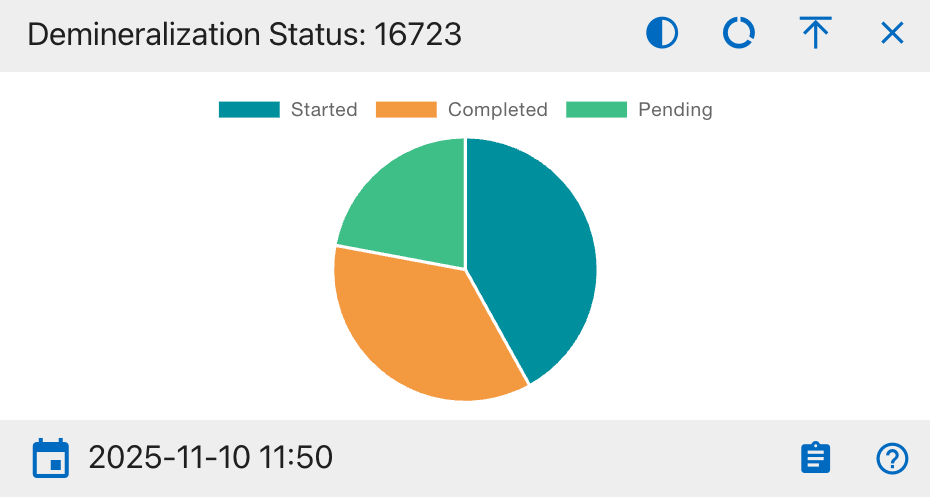
Pie Chart Segments:
- Started: Demineralization initiated.
- Completed: Process finished.
- Pending: Not started.
How to Use:
Confirm progress of sample preparation. High Completed means readiness for further processing.
Vial Weight Measurements
Purpose:
Monitors vial-based weighing consistency.
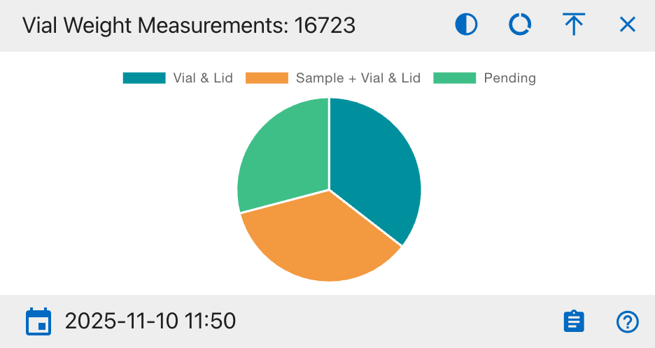
Pie Chart Segments:
- Vial & Lid: Empty container weight.
- Sample + Vial & Lid: Sample included weight.
- Pending: Measurements not done.
How to Use:
Used for verifying pre- and post weighting consistency to ensure analytical accuracy.
Collagen Measurements
Purpose:
Shows extracted collagen weight and yield.
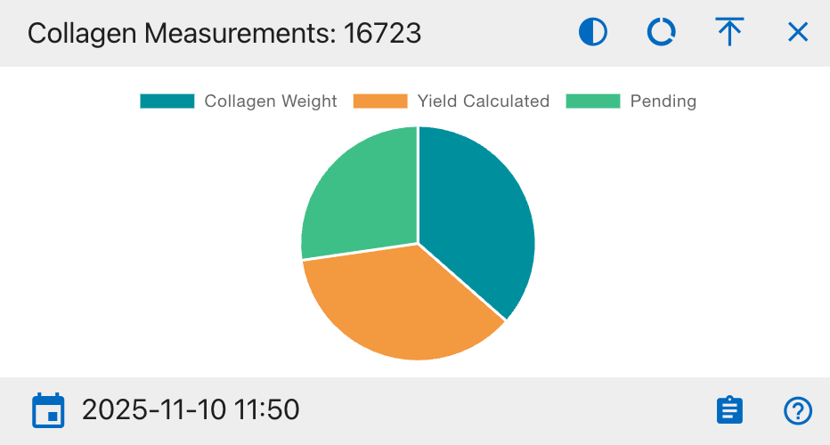
Pie Chart Segments:
- Collagen Weight: Extracted weight recorded.
- Yield Calculated: Yield percentage computed.
- Pending: Not yet completed.
How to Use:
Tracks collagen recovery efficiency. High Pending means incomplete or delayed extractions.
Carbon/Nitrogen Ratio (C:N)
Purpose:
Evaluates collagen preservation via C:N ratio.
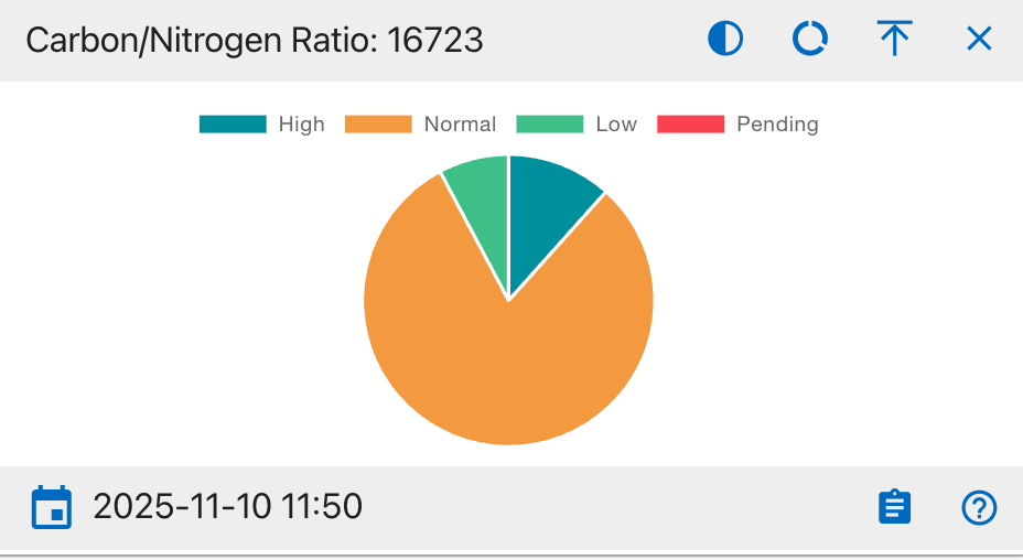
Pie Chart Segments:
- High (>3.6): Indicates contamination or degradation.
- Normal (2.9–3.6): Ideal preservation range.
- Low (<2.9): Possible underprocessing.
- Pending: Ratio not computed.
How to Use:
Healthy samples fall mostly under Normal. Alerts if ratio trends deviate.
Carbon/Oxygen Ratio (C:O)
Purpose:
Analyzes isotopic stability via C:O ratio.
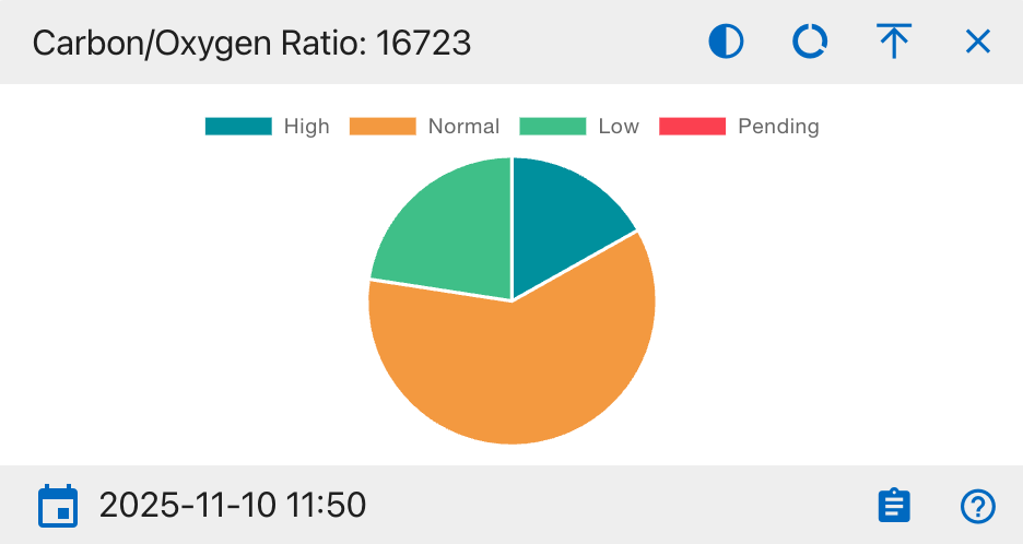
Pie Chart Segments:
- High (>1.4): Oxygen deficiency.
- Normal (1.1–1.4): Balanced.
- Low (<1.1): Oxygen rich contamination.
- Pending: Not calculated.
How to Use:
Used for consistency checks in isotope balance assessments.
Sample Results Status
Purpose: Displays overall isotope sample distribution by result status for tracking analytical completion.
Pie Chart Segments:
- Reportable: Verified isotopic results ready for reporting.
- Inconclusive: Data analyzed but not definitive.
- Unable to Assign: Insufficient data to categorize.
- Pending: Samples awaiting processing.
How to Use: Monitor lab analysis completion and identify pending or inconclusive samples. A higher Reportable ratio indicates improved analysis progress.
Weight Analysis Status
Purpose: Shows progress of sample weighing during isotope preparation.
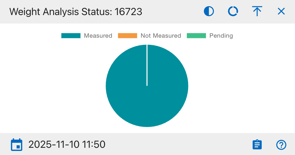
Pie Chart Segments:
- Measured: Samples successfully weighed.
- Not Measured: Samples yet to be weighed.
- Pending: Awaiting confirmation or data entry.
How to Use: Use this chart to verify weighing consistency and data completeness before analysis. A high Measured ratio indicates accurate preparation workflow.
Carbon Analysis (δ¹³C)
Purpose:
Visualizes completeness of carbon isotopic readings.
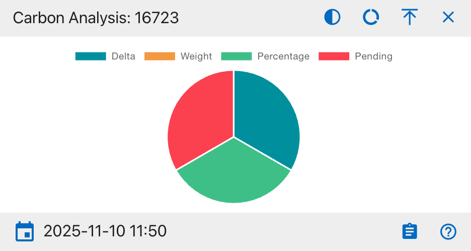
Pie Chart Segments:
- Delta (δ¹³C): Delta value recorded.
- Weight: Carbon weight data present.
- Percentage: Percent value entered.
- Pending: Missing carbon data.
How to Use:
Ensures all carbon-related fields are filled before analysis.
Nitrogen Analysis (δ¹⁵N)
Purpose:
Displays nitrogen isotope data completeness.
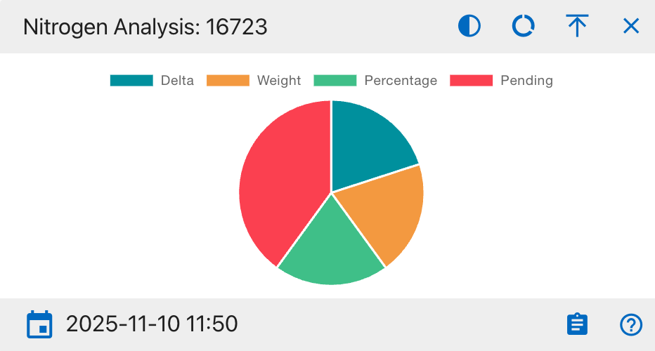
Pie Chart Segments:
- Delta (δ¹⁵N): Delta measured.
- Weight: Weight recorded.
- Percentage: Percent recorded.
- Pending: Incomplete nitrogen data.
How to Use:
Used by analysts studying dietary or ecological nitrogen variations.
Oxygen Analysis (δ¹⁸O)
Purpose:
Shows isotopic completeness for oxygen.
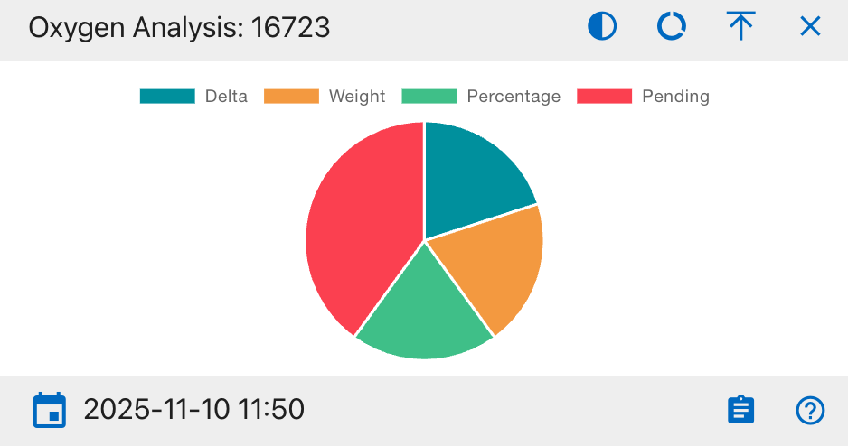
Pie Chart Segments:
- Delta (δ¹⁸O): Delta recorded.
- Weight: Weight recorded.
- Percentage: Percentage calculated.
- Pending: Missing oxygen data.
How to Use:
Ensures oxygen-related readings are sufficient for isotopic comparison.
Sulphur Analysis (δ³⁴S)
Purpose:
Summarizes sulphur isotope analysis results.
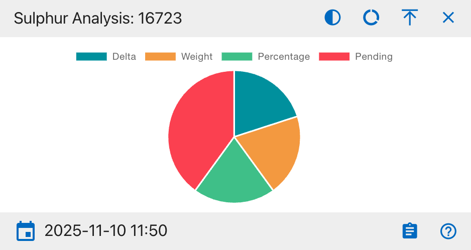
Pie Chart Segments:
- Delta (δ³⁴S): Delta measured.
- Weight: Weight captured.
- Percentage: Percent value recorded.
- Pending: Awaiting analysis.
How to Use:
Helps evaluate trace element (sulphur) data completeness.
Isotopes (Line Chart)
Purpose:
Displays time-based progress of isotope sample processing.
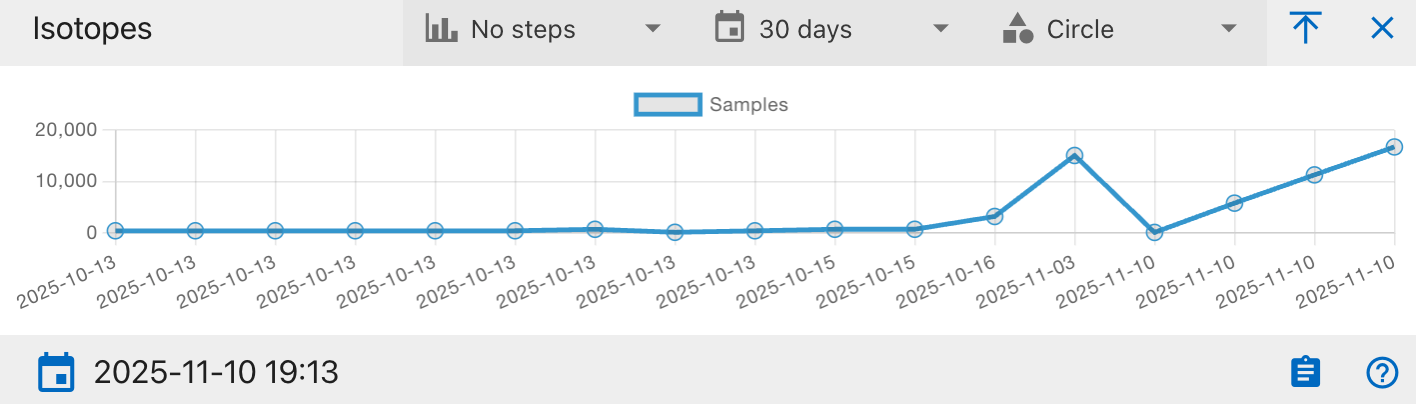
Chart Axes:
- X-Axis: Processing or entry date.
- Y-Axis: Number of analyzed samples.
How to Use:
Used to track throughput trends or identify bottlenecks.
Missing Person Dashboard
The Missing Person Dashboard provides a centralized interface for tracking, visualizing, and analyzing all Missing Person records within CoRA. It helps organization administrators and case managers to view key statistics and quickly access details for ongoing cases.
Navigation
To access the Missing Person Dashboard, use the left sidebar and select 'Missing Person Dashboard' under the Missing Person section. The dashboard will appear with various widgets and visual summaries.

Dashboard Overview
The Missing Person Dashboard provides visual insights into the status and progress of missing persons cases through a variety of widgets. These include pie charts and bar graphs that display case statuses, genealogical statuses, conflict categories, and case manager workloads. Each widget is interactive, allowing users to view detailed data, apply filters, and drill into specific case information. This centralized dashboard supports efficient case management and monitoring for organization administrators and case managers.
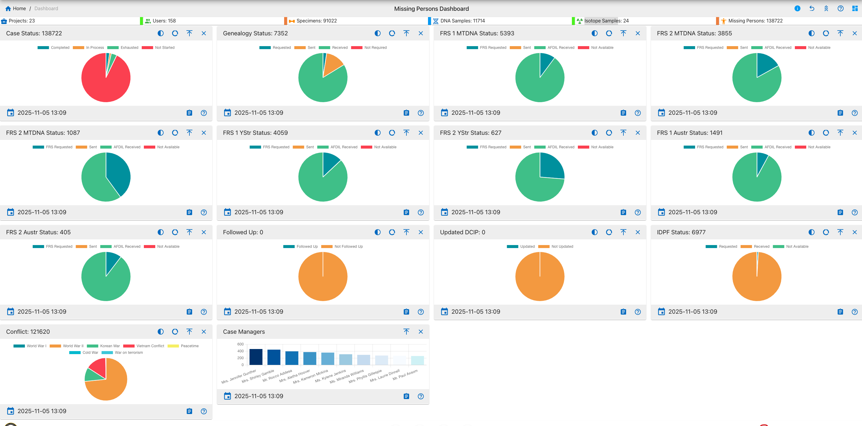
This dashboard provides essential tools to support effective case management and monitoring of missing persons within organization. For further information, detailed instructions, and troubleshooting, please refer to the comprehensive help documentation.
Widget Controls & Interactive Features
This dashboard supports the following user interactions and controls:
Common Controls
- Expand, Collapse & Close - Adjust widget layout for optimal viewing.
- Help/Info Icon - Access widget usage details and documentation links.
Interactivity
- Hover for Details - Move your mouse over chart segments or bars to view tooltips and counts.
- Drill Down - Click chart elements to reveal detailed tables or filtered records for deeper investigation.
Data Operations
- Export - Download data tables to Excel or PDF using icons above each table.
- Column Visibility - Choose which data columns to display.
- Search & Filter - Use the built-in table search for rapid filtering.
Data Freshness
- Timestamp - A 'Last Updated' timestamp is shown below each widget, so you can confirm the data is up to date.

Chart Visualization Types
The dashboard uses three main types of charts: full pie charts, which display a complete 360-degree representation of category proportions; half pie charts, which offer a compact semicircular visualization suitable for binary comparisons or space-constrained layouts; and donut charts, which emphasize individual segments while providing space in the center for additional information or layered data. Each chart type supports interactive features like hover tooltips and click-through details for enhanced user engagement.
Widget Details
Below is a detailed description of each widget included in the Missing Person Dashboard, their purpose, and interaction capabilities.
Case Status
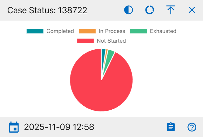
The details shown include:
- Completed
- In Process
- Exhausted
- Not Started
This widget provides a visual breakdown of all missing person case statuses within the organization. The pie chart displays the proportion of cases that are completed, in process, exhausted, or not started. Users can hover over segments for further data and click to export the supporting table to Excel or PDF. Filters and column visibility options are available in the integrated data table beneath the chart.
Genealogy Status
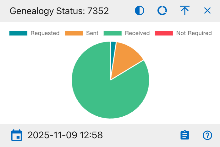
The details shown include:
- Requested
- Sent
- Received
- Not Required
This widget displays the current genealogy status for missing person cases. The pie chart segments represent the cases that have been requested, sent, received, or do not require genealogy updates. Users can hover over segments for further data and click to export the supporting table to Excel or PDF. Filters and column visibility options are available in the integrated data table beneath the chart.
FRS 1 MTDNA Status

The details shown include:
- FRS Requested
- Sent
- AFDIL Received
- Not Available
This widget displays the status distribution of the first Family Reference Sample (MTDNA) requests for all missing person cases. The pie chart sections represent the proportion of samples that are requested, sent, received by AFDIL, or not available. Users can hover over segments for further data and click to export the supporting table to Excel or PDF. Filters and column visibility options are available in the integrated data table beneath the chart.
FRS 2 MTDNA Status

The details shown include:
- FRS Requested
- Sent
- AFDIL Received
- Not Available
This widget displays the status distribution for the second Family Reference Sample (MTDNA) requests in missing person cases. Users can hover over segments for further data and click to export the supporting table to Excel or PDF. Filters and column visibility options are available in the integrated data table beneath the chart.
FRS 3 MTDNA Status
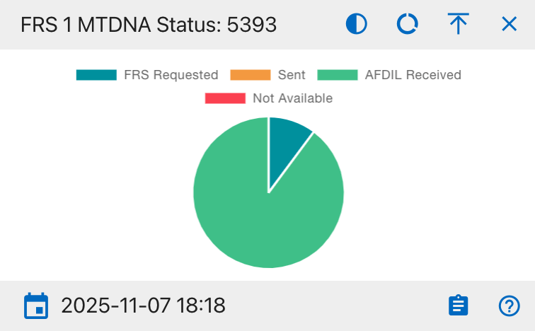
- FRS Requested
- Sent
- AFDIL Received
- Not Available
This widget displays the status of the third Family Reference Sample (MTDNA) requests for missing person cases. Users can hover over segments for further data and click to export the supporting table to Excel or PDF. Filters and column visibility options are available in the integrated data table beneath the chart.
FRS 1 YStr Status

- FRS Requested
- Sent
- AFDIL Received
- Not Available
This widget displays the status of the first Family Reference Sample (YStr) requests for missing person cases. Users can hover over segments for further data and click to export the supporting table to Excel or PDF. Filters and column visibility options are available in the integrated data table beneath the chart.
FRS 2 YStr Status
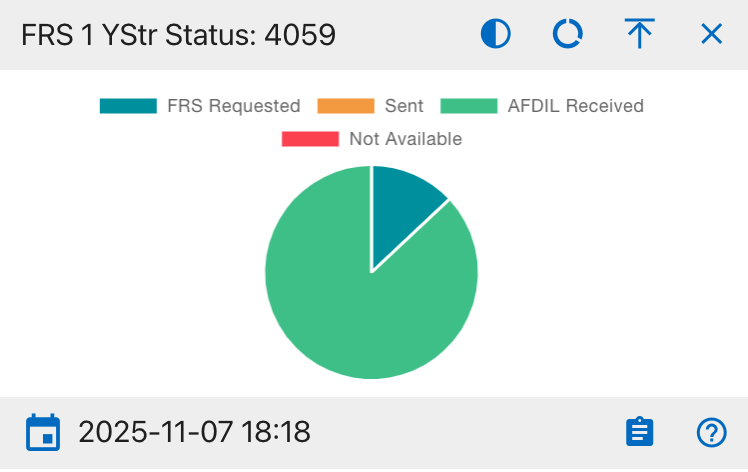
- FRS Requested
- Sent
- AFDIL Received
- Not Available
This widget provides the status distribution for the second Family Reference Sample (YStr) requests in missing person cases. Users can hover over segments for further data and click to export the supporting table to Excel or PDF. Filters and column visibility options are available in the integrated data table beneath the chart.
FRS 1 AUSTR Status
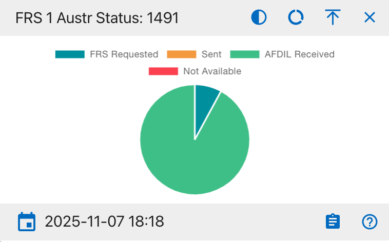
- FRS Requested
- Sent
- AFDIL Received
- Not Available
This widget displays the status breakdown of the first Family Reference Sample (AUSTR) requests for missing person cases. Users can hover over segments for further data and click to export the supporting table to Excel or PDF. Filters and column visibility options are available in the integrated data table beneath the chart.
FRS 2 AUSTR Status
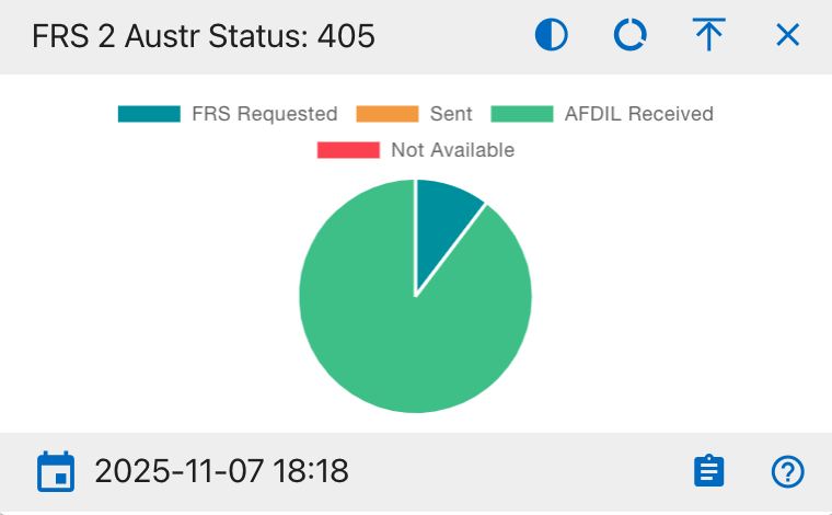
- FRS Requested
- Sent
- AFDIL Received
- Not Available
This widget displays the status breakdown of the second Family Reference Sample (AUSTR) requests for missing person cases. Users can hover over segments for further data and click to export the supporting table to Excel or PDF. Filters and column visibility options are available in the integrated data table beneath the chart.
Followed Up
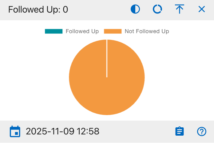
- Followed Up
- Not Followed Up
This widget displays the proportion of missing person cases that have been followed up by a case manager. Users can hover over segments for further data and click to export the supporting table to Excel or PDF. Filters and column visibility options are available in the integrated data table beneath the chart.
Updated DCIP
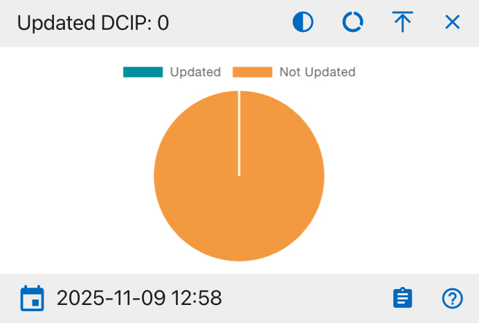
- Updated
- Not Updated
This widget displays how many missing person cases have their DCIP records updated versus not updated. Users can hover over segments for further data and click to export the supporting table to Excel or PDF. Filters and column visibility options are available in the integrated data table beneath the chart.
IDPF Status
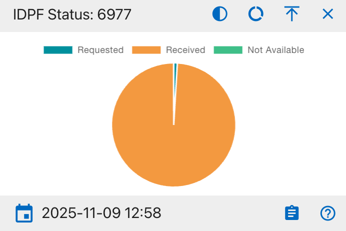
The details shown include:
- Requested
- Received
- Not Available
This widget displays the status of IDPF (Individual Deceased Personnel File) requests for missing person cases. The pie chart shows the number of requests in each state (Requested, Received, Not Available). Users can hover over segments for further data and click to export the supporting table to Excel or PDF. Filters and column visibility options are available in the integrated data table beneath the chart.
Conflict
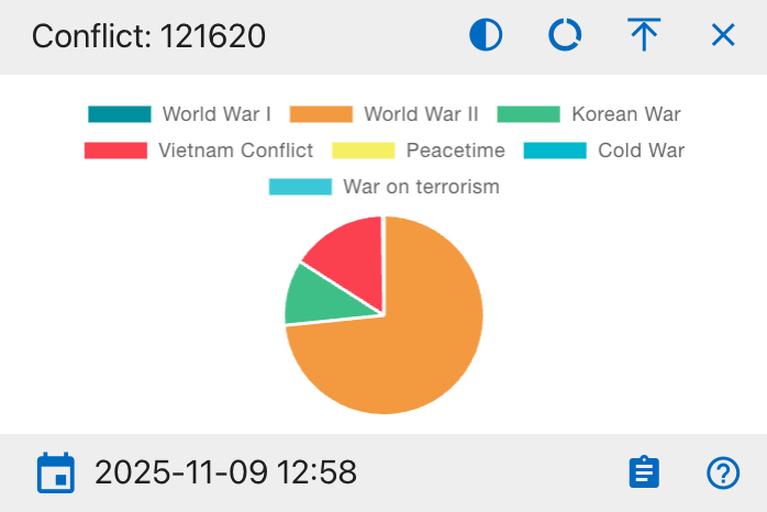
The details shown include:
- World War I
- World War II
- Korean War
- Vietnam Conflict
- Peacetime
- Cold War
- War on Terrorism
This widget visualizes missing person cases by conflict type. Each segment represents the number of cases from a particular conflict era. Users can hover over segments for further data and click to export the supporting table to Excel or PDF. Filters and column visibility options are available in the integrated data table beneath the chart.
Case Managers
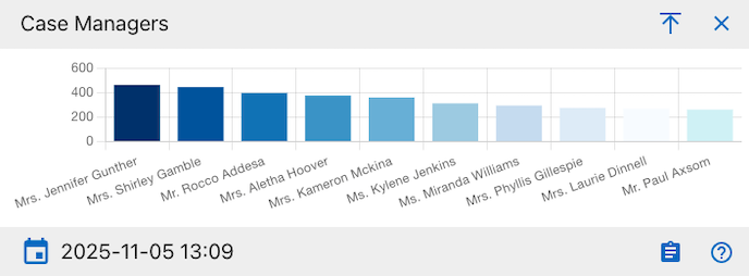
The details shown include:
- Case Manager name
- Total number of cases assigned
This widget displays the number of missing person cases assigned to each case manager using a horizontal bar chart. Each bar represents an individual case manager, with the height indicating their total case load. Users can hover over bars for further data and click to export the supporting table to Excel or PDF. Filters and column visibility options are available in the integrated data table beneath the chart.
User Dashboard
Warning
This page is work in progress.
The User Dashboard serves as a high level view of both summary and aggregated user data.
User Activity
User activity contains widgets, which are individual visual representations of data. Examples of those widgets include:
- Skeletal Elements Assocciated To Individual
- DNA Sample Information
Those widgets can be added and removed via the widget selector. User activity widgets are present in the Org admin dashboards
On Click of key from the user activity widget present on dashboard shows the specimen page with details to edit and other actions.
On Click of details present on widgets, provides all the data for the selected module.
Below are the fields that are visible:
- Key
- Name
- Side
- Completeness
- Individual Number
- Measured
- Isotope Sampled
- Clavicle Triage
- CT Scanned
- Xray Scanned
- Inventoried
- Reviewed
- Inventoried At
- Reviewed At
- Created By
- Created At
- Updated By
- Updated At
These fields will vary depending on type of module selected
User Activity Specimen
Warning
This section is work in progress.
Org Dashboard
Warning
This page is work in progress.
The Org dashboard provides at a glance high level charts and tables of org data, information, statistics and charts for the current org.
Project Map
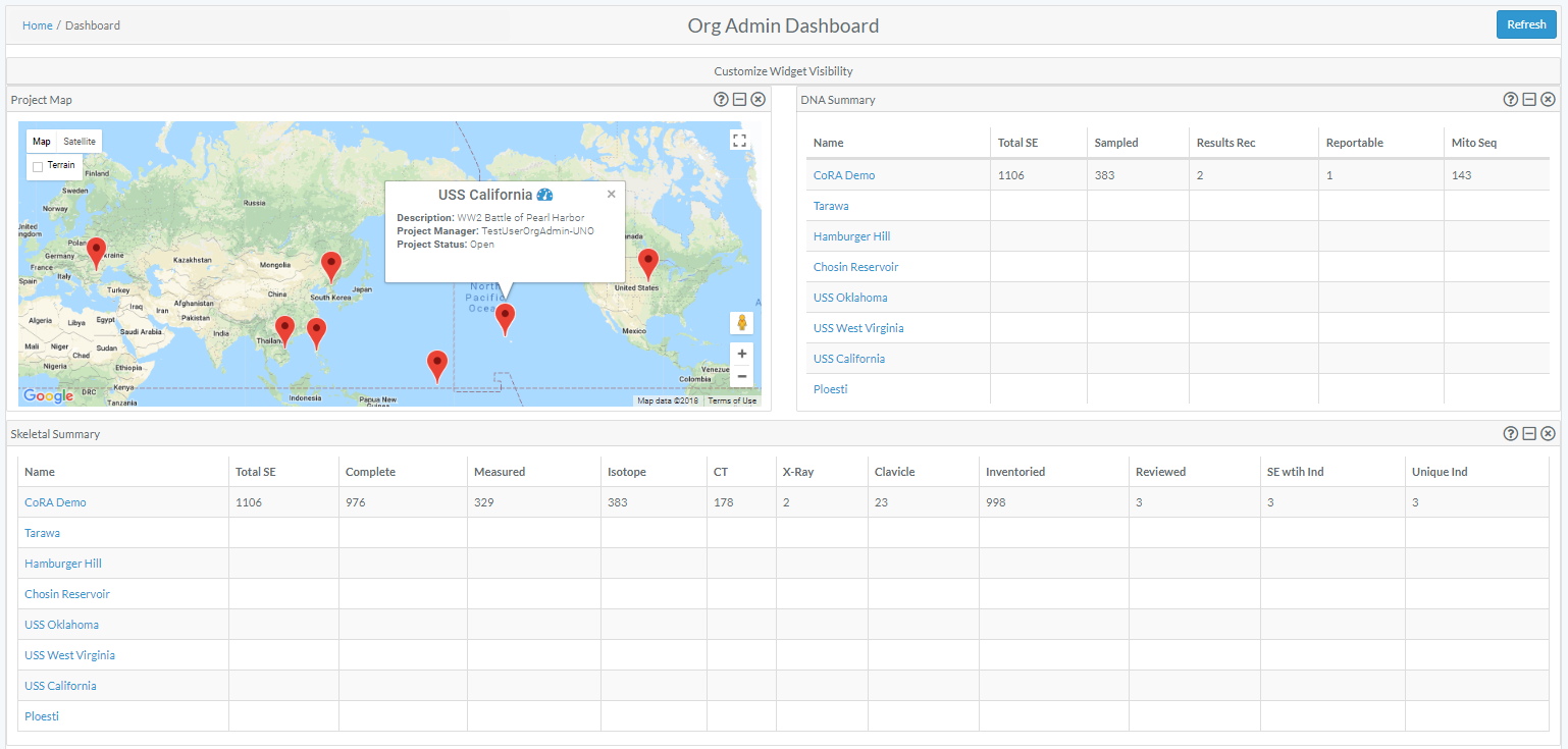
Markers
The markers displayed on the map showcase the latitude and longitude of a particular project.
On mouse over additional project details as well as a link ![]() to the corresponding project dashboard can be found in the in popup window.
to the corresponding project dashboard can be found in the in popup window.
Specimen Summary
A data table provides a link to a project dashboard and shows high level Skeletal Elements summary details for each project
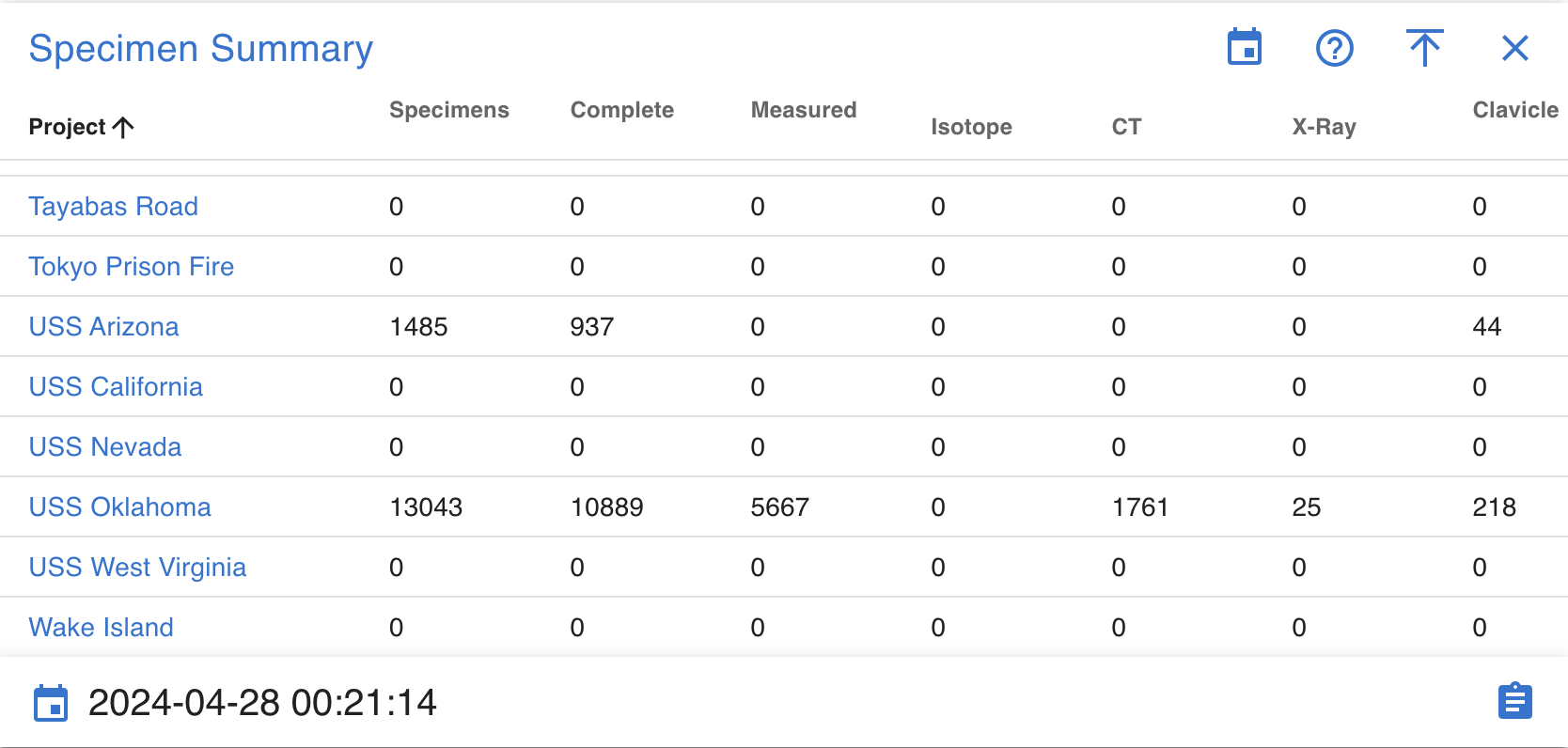
DNA Summary
A data table provides a link to a project dashboard and shows high level DNA summary details for each project
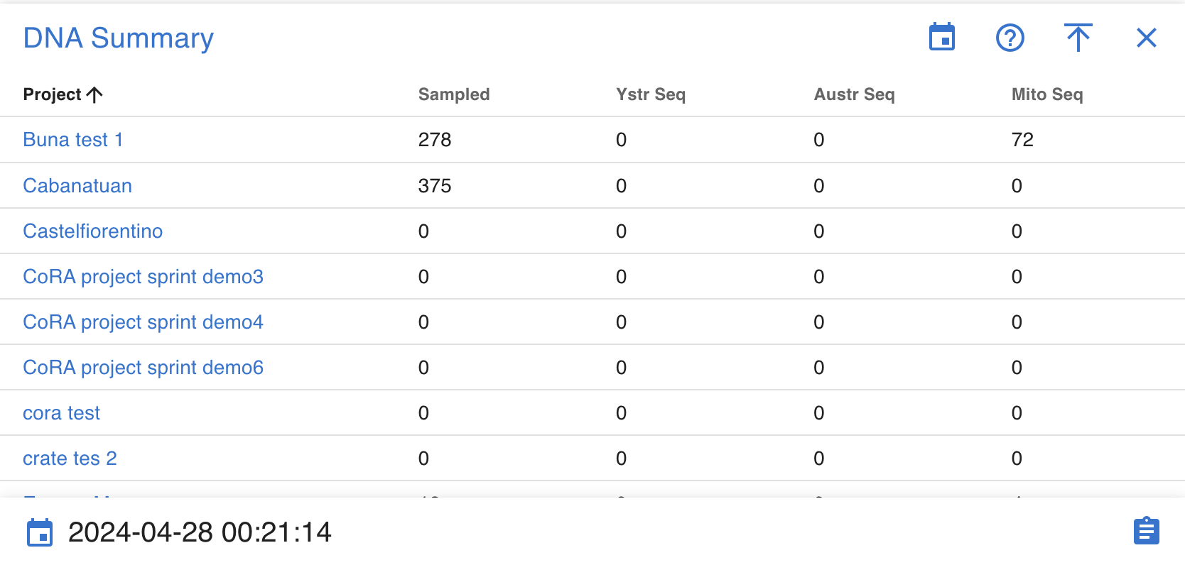
Isotope Summary
A data table provides a link to a project dashboard and shows high level Isotope summary details for each project
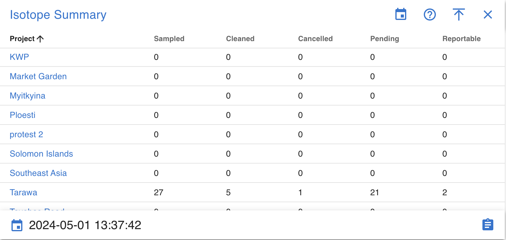
Missing Person Summary
A data table provides a link to a project dashboard and shows high level Missing Person summary details for each project
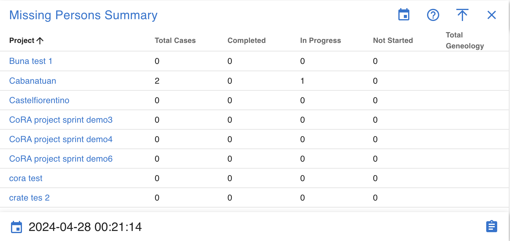
User Activity Specimen
Warning
This section is work in progress.
User Activity DNA
Warning
This section is work in progress.
Specimen Dashboard
Warning
This page is work in progress.
The Specimen dashboard provides information on the the charts and graphs from the dashboard.
Navigation
Warning
This section is work in progress.
Widget Features
Warning
This section is work in progress.
Complete
Warning
This section is work in progress.
Individual Assigned
Warning
This section is work in progress.
DNA Sampled
Warning
This section is work in progress.
Measured
Warning
This section is work in progress.
CT Scanned
Warning
This section is work in progress.
XRAY Scanned
Warning
This section is work in progress.
Clavicle Triage
Warning
This section is work in progress.
Isotope Sampled
Warning
This section is work in progress.
Remains Status
Warning
This section is work in progress.
Inventoried
Warning
This section is work in progress.
Reviewed
Warning
This section is work in progress.
Specimens
Warning
This section is work in progress.
Drilldowns
DNA Dashboard Drilldowns
This page documents the drilldown views available from the DNA Dashboard. Each drilldown provides detailed tabular data corresponding to a specific DNA analysis metric or category. Users can search, filter, sort, and export data from these views.
Navigation
Click on detail button on any chart widget in the DNA Dashboard to access its corresponding drilldown page. Each drilldown displays a visual representation of the data at the top, followed by a detailed data table below.
Available Actions
-
Search - Use the search bar at the top of any column to find specific samples by entering text in the search fields
-
Sort - Click any column header to sort data in ascending or descending order for easy data organization
-
Export - Download the filtered data in multiple formats:
- Excel - Export to Excel spreadsheet for advanced analysis
- PDF - Generate a printable PDF report
- Column Visibility - Show or hide columns to customize your view by clicking the column visibility icon
- Pagination - Navigate through large datasets using the pagination controls at the bottom of the table
- Items per Page - Adjust the number of rows displayed (25, 50, 100) using the dropdown menu
- View Details - Click on any row to view complete DNA sample information and related specimen details
- Refresh Data - Click the refresh icon to reload the table with the most current data
Mitochondrial DNA (Mito) Drilldowns
Table Fields
- Key - Unique record identifier assigned to each DNA sample entry in the system for tracking and reference purposes
- Bone - Skeletal bone element name indicating the specific bone from which the DNA sample was collected (e.g., Femur, Humerus, Tibia)
- Side - Anatomical side designation showing whether the bone is from the Left or Right side of the body
- Bone Group - Bone classification category grouping similar bones together for organizational and analytical purposes (e.g., Long Bones, Skull, Ribs)
- Individual Number - Associated individual identifier linking the DNA sample to a specific person or skeletal remains for identification purposes
- Sample Number - DNA sample identifier serving as the primary unique reference number for the specific DNA sample collected
- External Case ID - External case reference number used by outside agencies or laboratories to track the case
- External Sample Number - External sample reference number assigned by external laboratories or agencies for their tracking purposes
- Mito Sequence Number - Mitochondrial DNA sequence identifier representing the unique mtDNA profile assigned after analysis
- Mito Sequence Subgroup - Mitochondrial sequence subcategory providing additional classification detail within the main sequence group
- Mito Sequence Similar - Similar mitochondrial sequences showing other samples that share matching or closely related mtDNA profiles
- Mito Receive Date - Date mitochondrial DNA results were received from the laboratory, marking when analysis was completed
DNA Mito Results
The DNA Mito Results drilldown displays all DNA samples that have mitochondrial DNA (mtDNA) result confidence levels recorded. This view helps track the quality and reliability of mitochondrial DNA analysis results across samples.
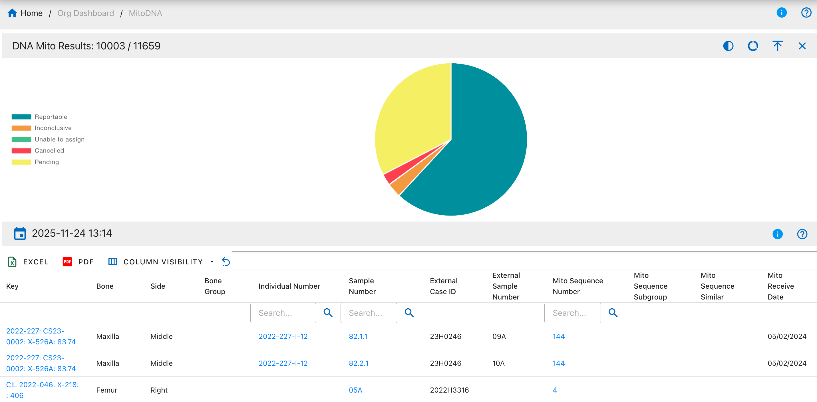
Pie Chart Segments:
- Reportable
- Inconclusive
- Unable to assign
- Cancelled
- Pending
DNA Mito Methods
The DNA Mito Methods drilldown shows all DNA samples categorized by the laboratory method used for mitochondrial DNA sequencing analysis.
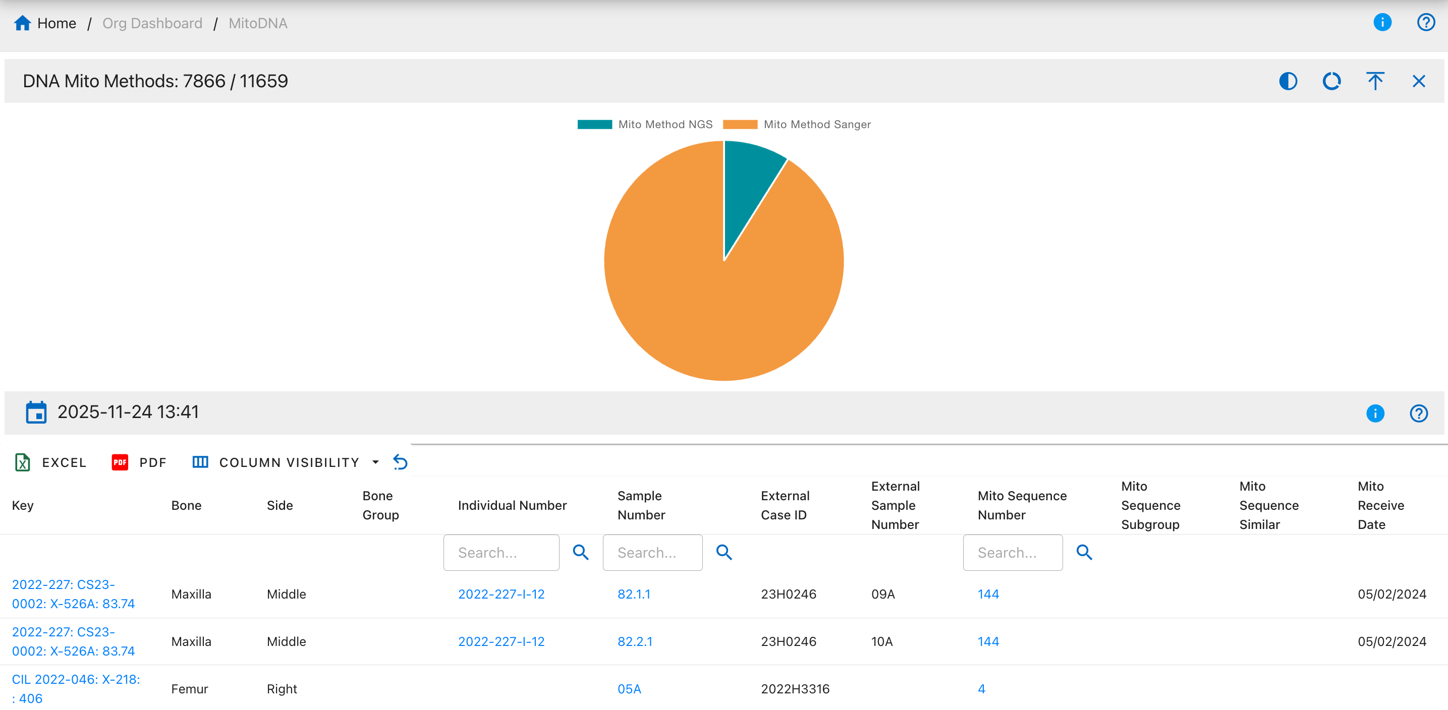
Pie Chart Segments:
- Mito Method NGS
- Mito Method Sanger
DNA Mito Counts
The DNA Mito Counts drilldown displays DNA samples with recorded match count and total count data, showing how many specimens share the same mitochondrial DNA sequence.
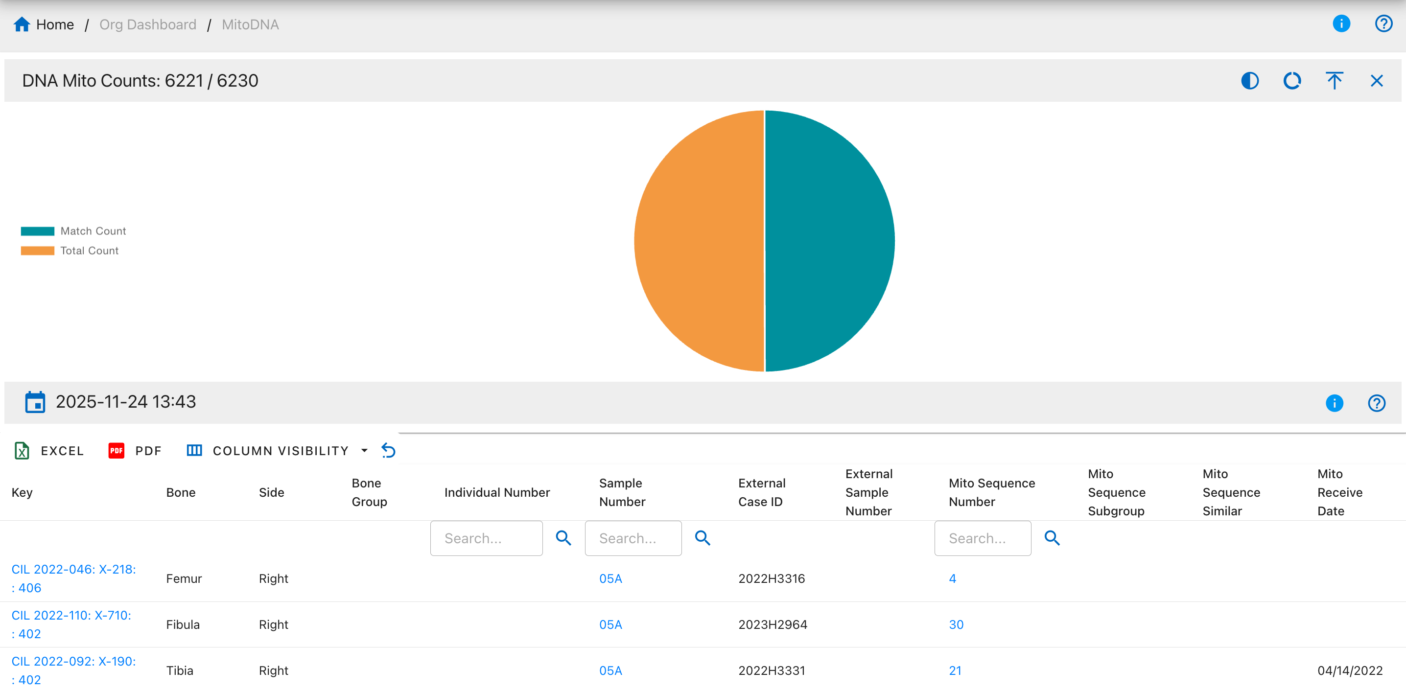
Pie Chart Segments:
- Match Count
- Total Count
DNA Mito Dates
The DNA Mito Dates drilldown shows all DNA samples with recorded mitochondrial DNA request and receive dates, helping track turnaround times and lab processing schedules.
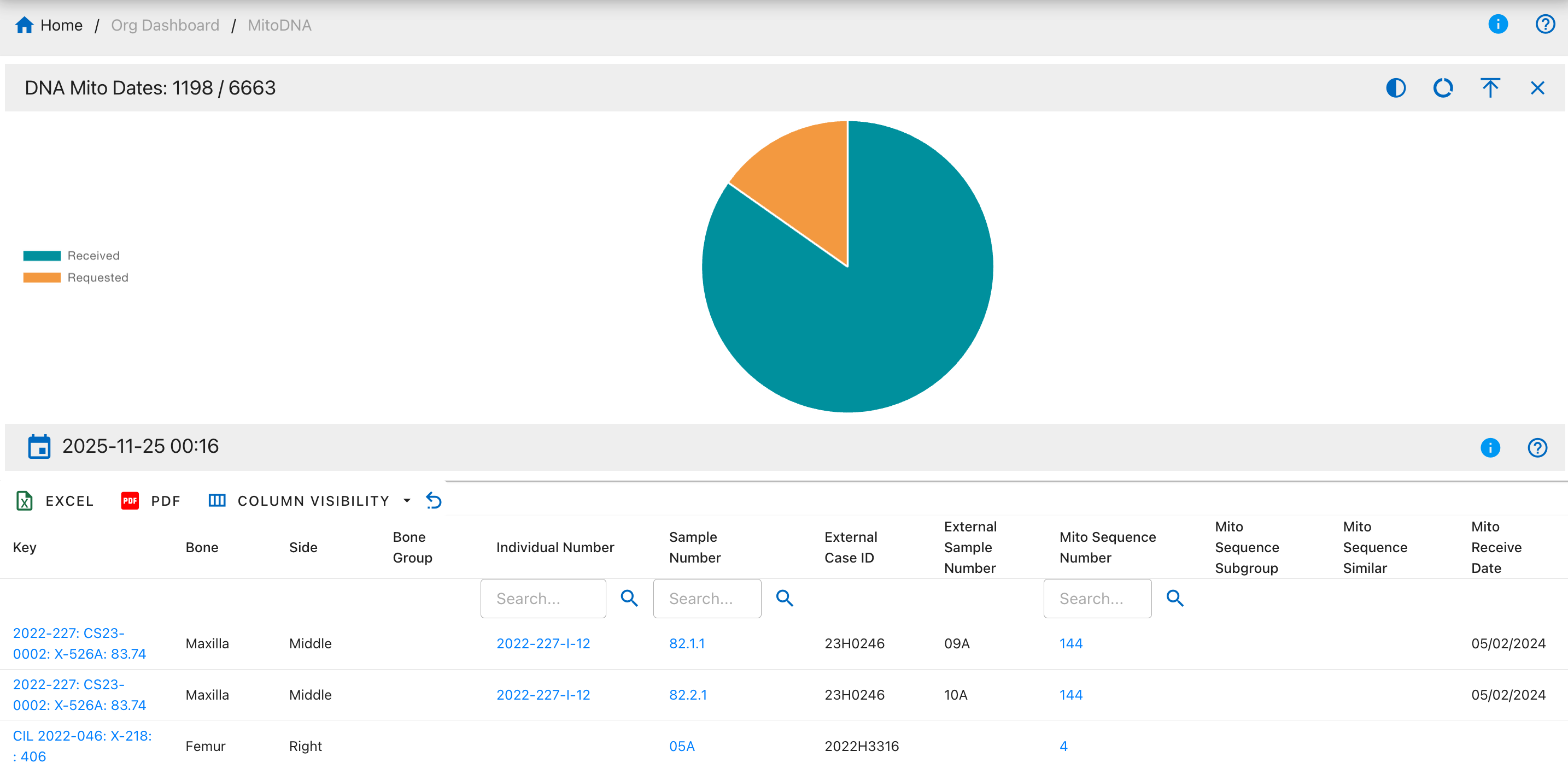
Pie Chart Segments:
- Received
- Requested
DNA Mito Sequence
The DNA Mito Sequence drilldown displays samples with assigned mitochondrial DNA sequence numbers, allowing tracking of unique mtDNA profiles across specimens.

Pie Chart Segments:
- Number
- Subgroup
- Similar
DNA Mito Haplogroup
The DNA Mito Haplogroup drilldown shows DNA samples categorized by their mitochondrial haplogroup classification, representing maternal lineage.

Pie Chart Segments:
- Assigned
- Not Assigned
DNA Mito Confirmed Regions
The DNA Mito Confirmed Regions drilldown displays samples with confirmed mitochondrial DNA sequence regions that have been verified through analysis.
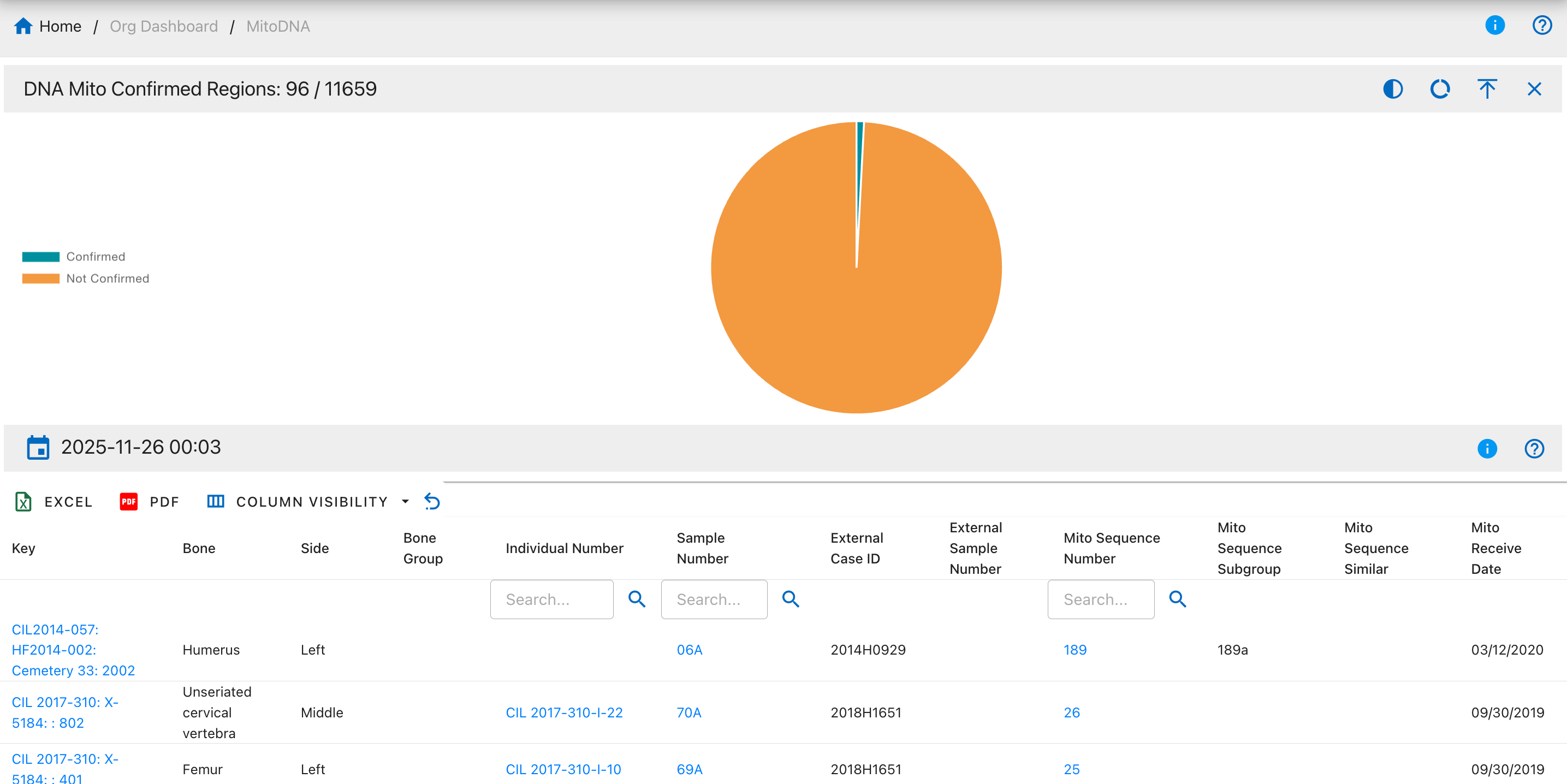
Pie Chart Segments:
- Confirmed
- Not Confirmed
DNA Mito Base Pairs
The DNA Mito Base Pairs drilldown shows DNA samples with recorded mitochondrial DNA base pair information, indicating the specific nucleotide positions analyzed.

Pie Chart Segments:
- Sequenced
- Not Sequenced
DNA Mito Polymorphisms
The DNA Mito Polymorphisms drilldown displays samples with recorded mitochondrial DNA polymorphisms (sequence variations).
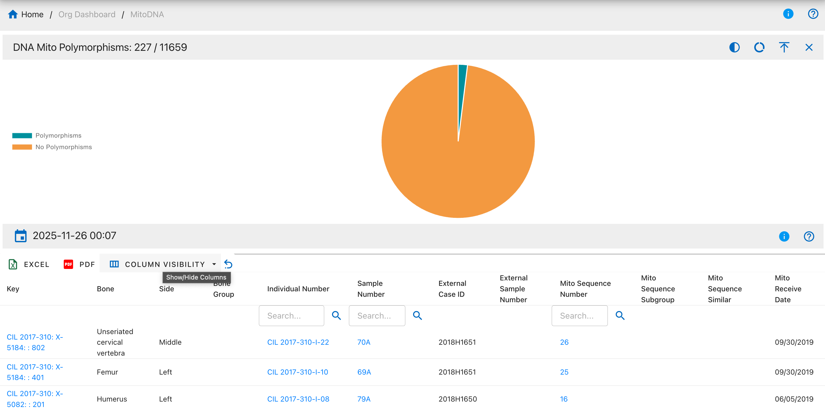
Pie Chart Segments:
- Polymorphisms
- No Polymorphisms
DNA Mito FASTA Sequence
The DNA Mito FASTA Sequence drilldown shows samples with complete FASTA-formatted mitochondrial DNA sequences available.
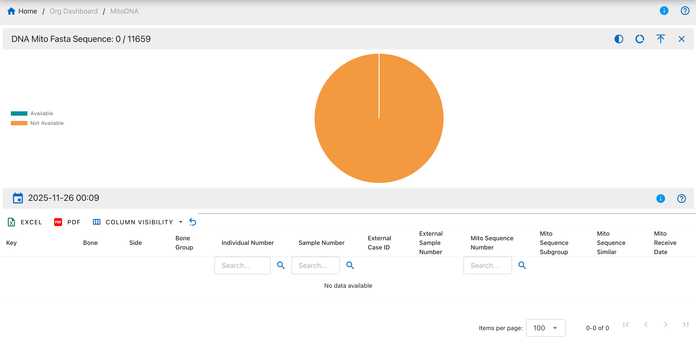
Pie Chart Segments:
- Available
- Not Available
DNA Mito Haplosubgroup
The DNA Mito Haplosubgroup drilldown displays samples with detailed mitochondrial haplosubgroup classifications, providing more specific maternal lineage information.
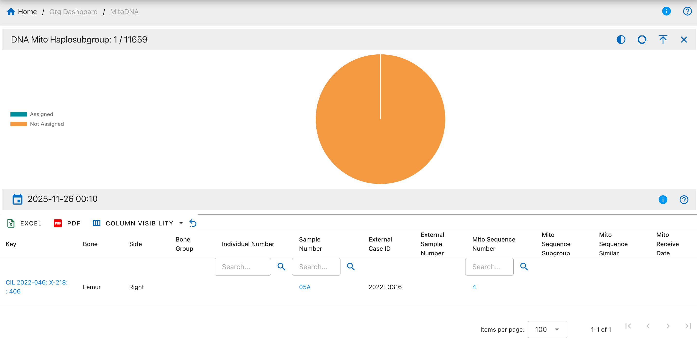
Pie Chart Segments:
- Assigned
- Not Assigned
DNA Mito Loci
The DNA Mito Loci drilldown shows DNA samples with information about specific mitochondrial DNA loci analyzed.
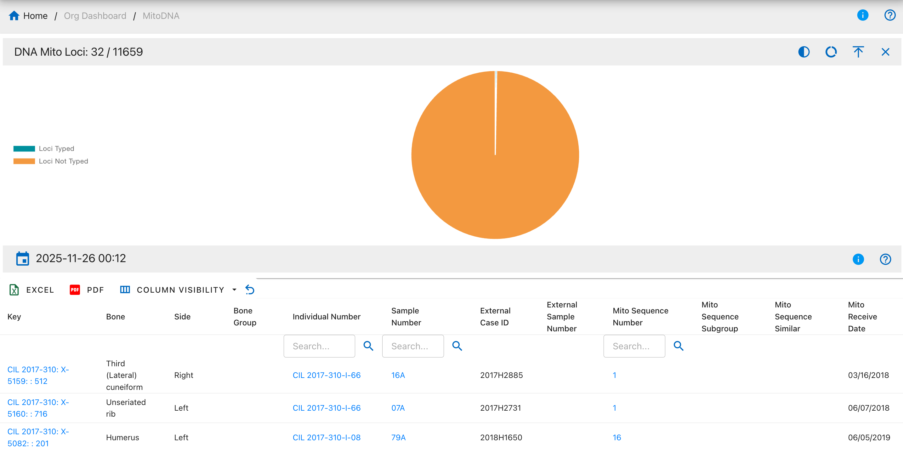
Pie Chart Segments:
- Loci Typed
- Loci Not Typed
DNA Mito MCC Dates
The DNA Mito MCC (Mitochondrial Control Region) Dates drilldown displays samples with MCC-specific request and receive dates.
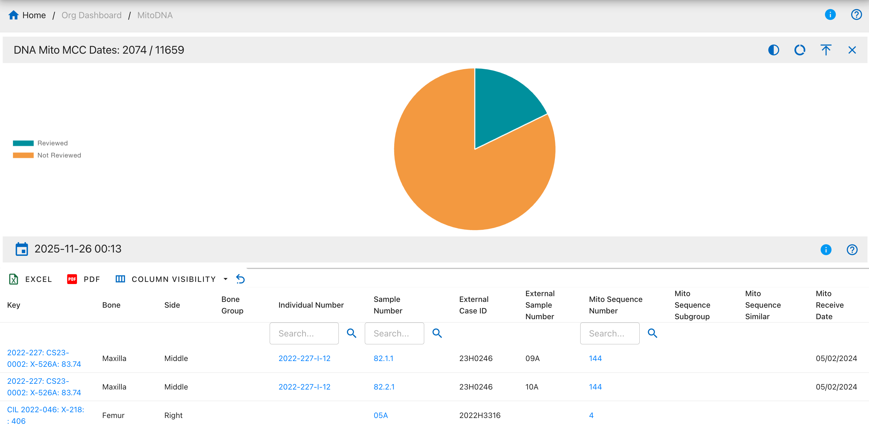
Pie Chart Segments:
- Reviewed
- Not Reviewed
DNA Sample Condition
The DNA Sample Condition drilldown displays the physical condition assessment of DNA samples at the time of collection or analysis.
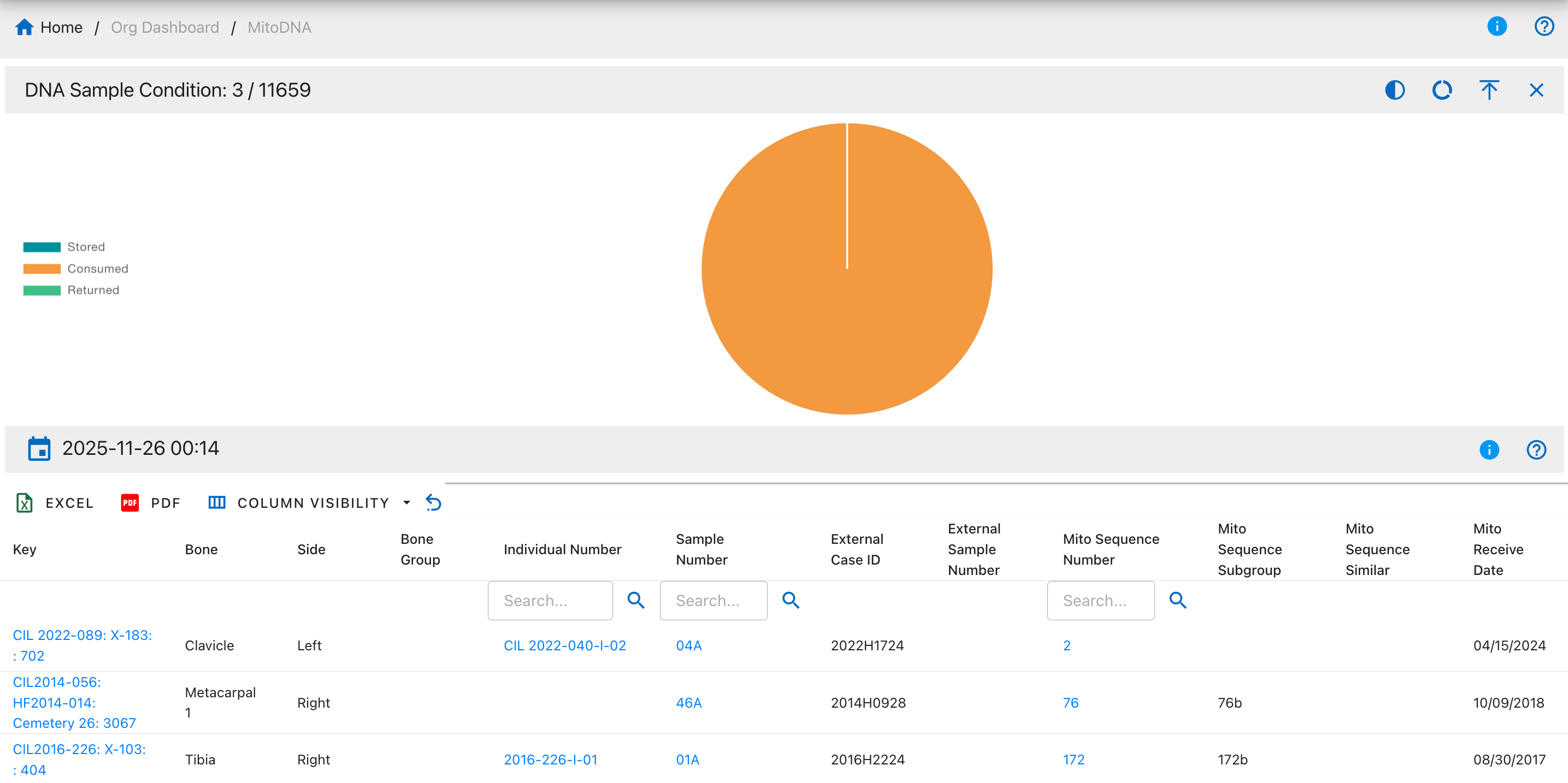
Pie Chart Segments:
- Stored
- Consumed
- Returned
DNA Resampled
The DNA Resampled drilldown shows samples that have been resampled for additional DNA analysis due to various reasons such as insufficient quality or quantity.

Pie Chart Segments:
- Resampled
- Not Resampled
DNA BTB Dates
The DNA Bone-to-Bone (BTB) Dates drilldown displays samples with bone-to-bone comparison request and receive dates, used for comparing DNA from multiple bones of the same individual.
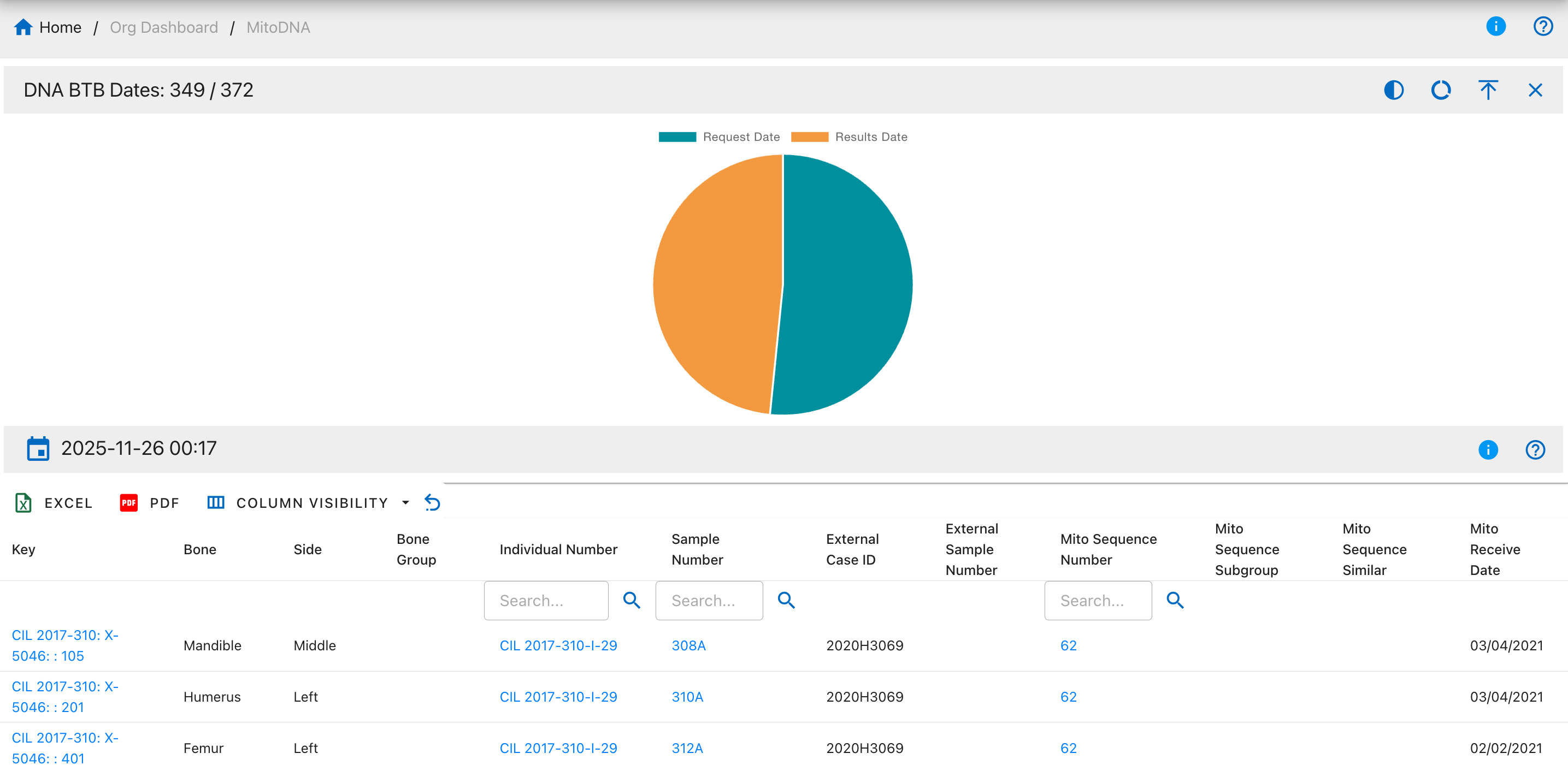
Pie Chart Segments:
- Request Date
- Results Date
Autosomal STR (AuSTR) Drilldowns
Table Fields
- Key - Unique record identifier assigned to each DNA sample entry in the system for tracking and reference purposes
- Bone - Skeletal bone element name indicating the specific bone from which the DNA sample was collected (e.g., Femur, Humerus, Tibia)
- Side - Anatomical side designation showing whether the bone is from the Left or Right side of the body
- Bone Group - Bone classification category grouping similar bones together for organizational and analytical purposes (e.g., Long Bones, Skull, Ribs)
- Individual Number - Associated individual identifier linking the DNA sample to a specific person or skeletal remains for identification purposes
- Sample Number - DNA sample identifier serving as the primary unique reference number for the specific DNA sample collected
- External Case ID - External case reference number used by outside agencies or laboratories to track the case
- External Sample Number - External sample reference number assigned by external laboratories or agencies for their tracking purposes
- AuSTR Sequence Number - Autosomal STR sequence identifier representing the unique autosomal DNA profile assigned after analysis
- AuSTR Sequence Similar - Similar autosomal STR sequences showing other samples that share matching or closely related profiles
- AuSTR Sequence Subgroup - Autosomal STR sequence subcategory providing additional classification detail within the main sequence group
- AuSTR Receive Date - Date autosomal STR DNA results were received from the laboratory, marking when analysis was completed
DNA AuSTR Methods
The DNA AuSTR Methods drilldown shows DNA samples categorized by the laboratory method used for autosomal STR analysis.
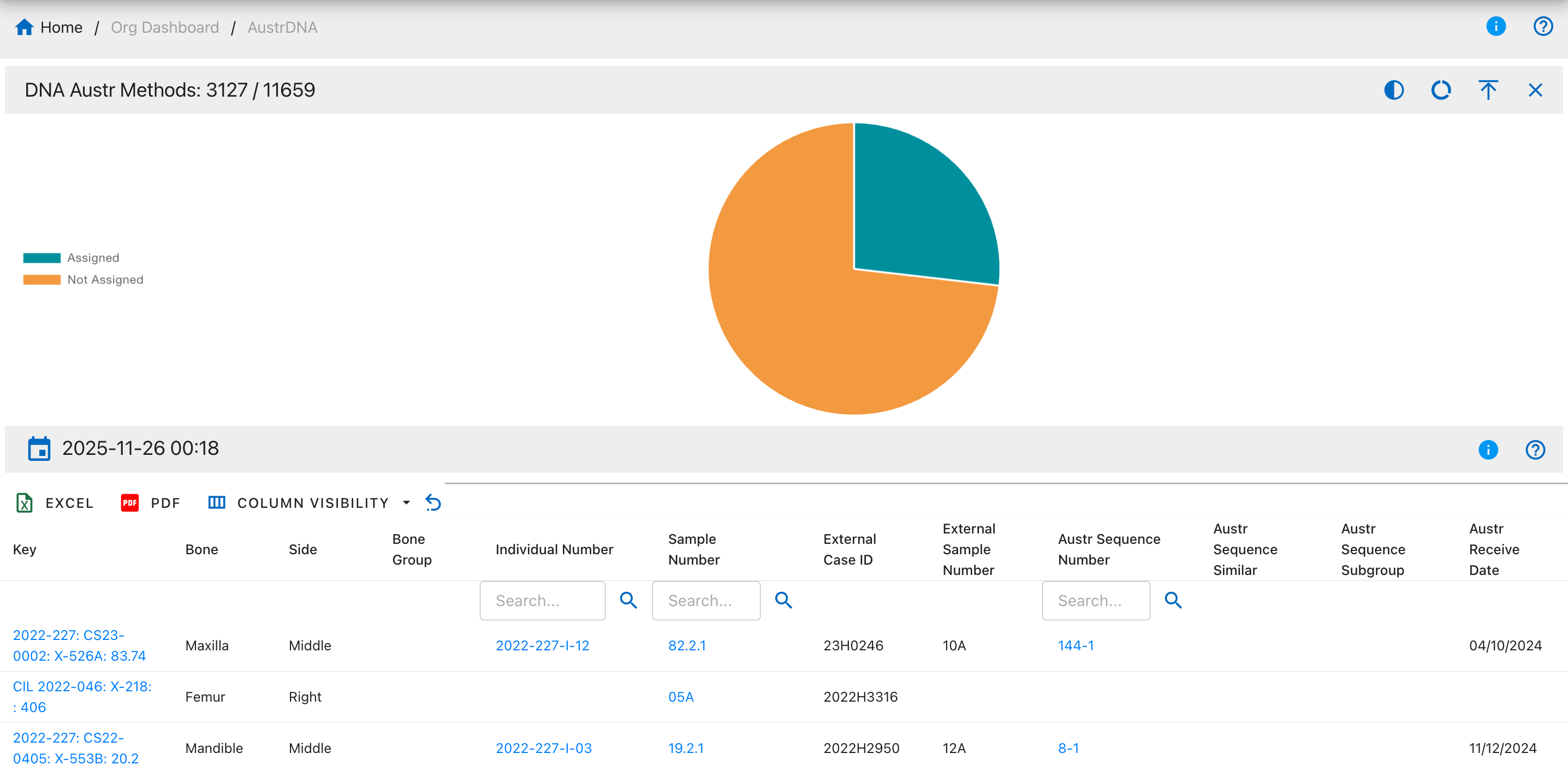
Pie Chart Segments:
- Assigned
- Not Assigned
DNA AuSTR Results
The DNA AuSTR Results drilldown displays all DNA samples with autosomal short tandem repeat (STR) analysis results.
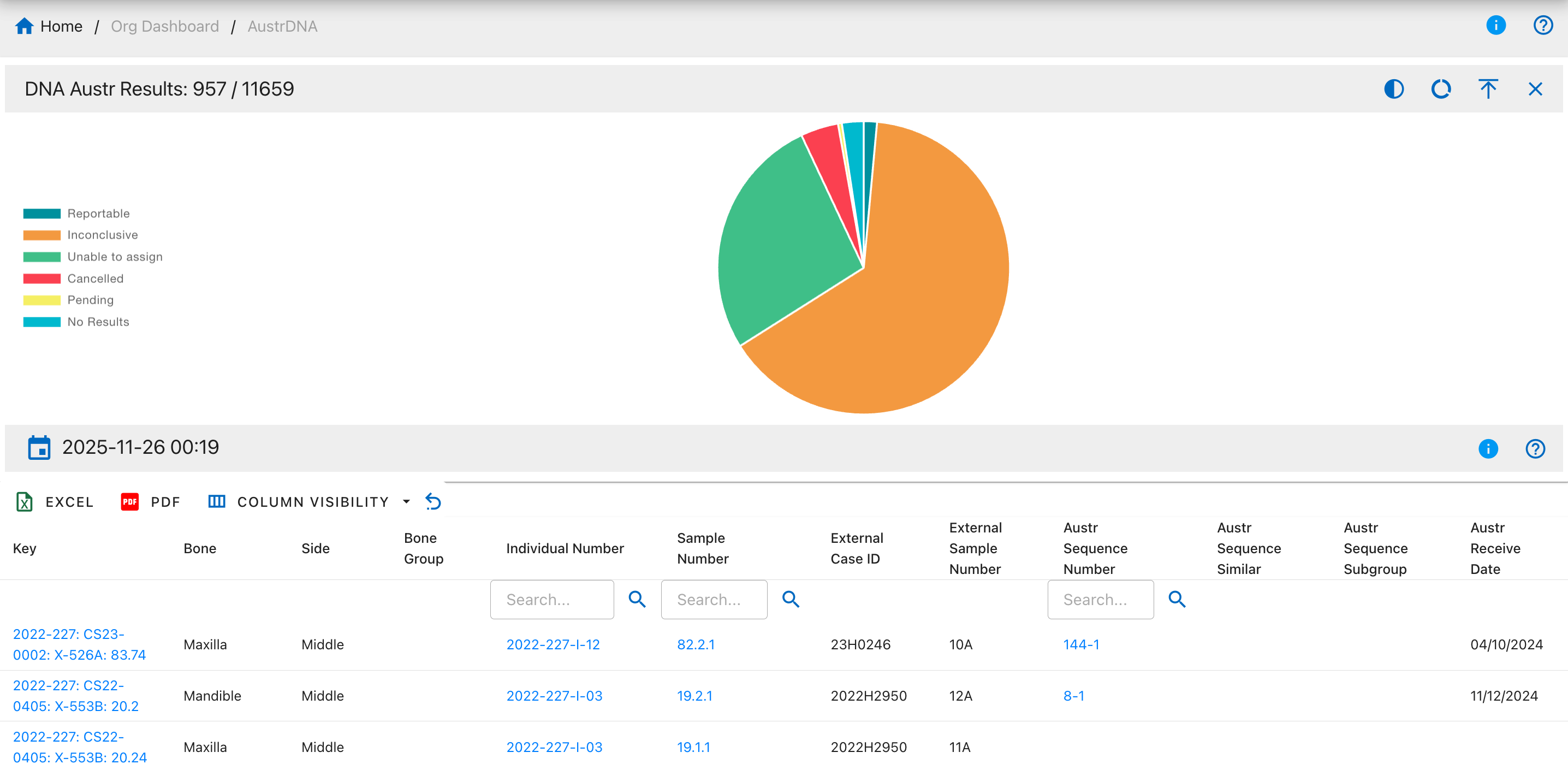
Pie Chart Segments:
- Reportable
- Inconclusive
- Unable to assign
- Cancelled
- Pending
- No Results
DNA AuSTR Dates
The DNA AuSTR Dates drilldown displays samples with autosomal STR request and receive dates.
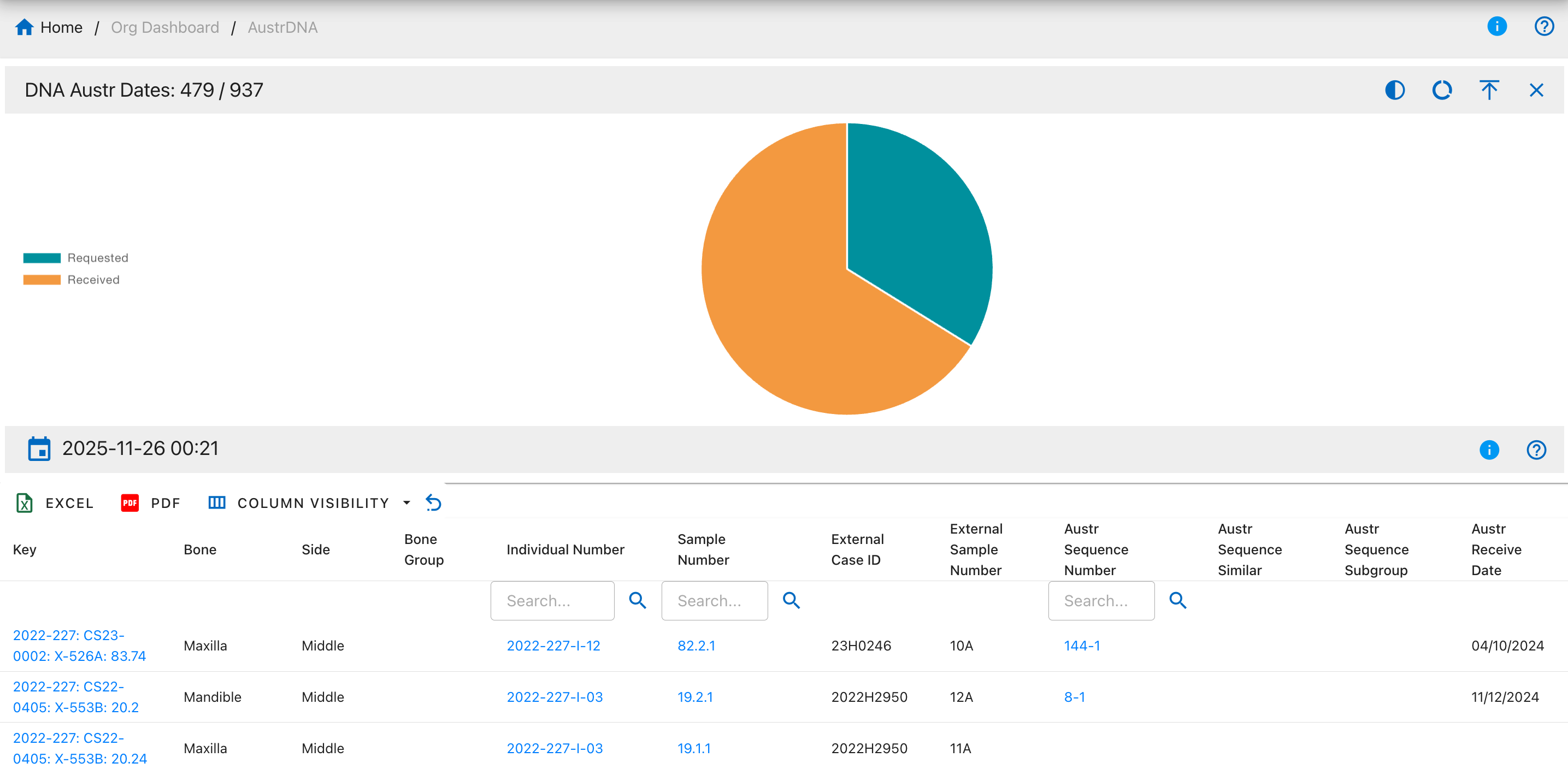
Pie Chart Segments:
- Requested
- Received
DNA AuSTR Sequence
The DNA AuSTR Sequence drilldown shows samples with assigned autosomal STR sequence numbers.
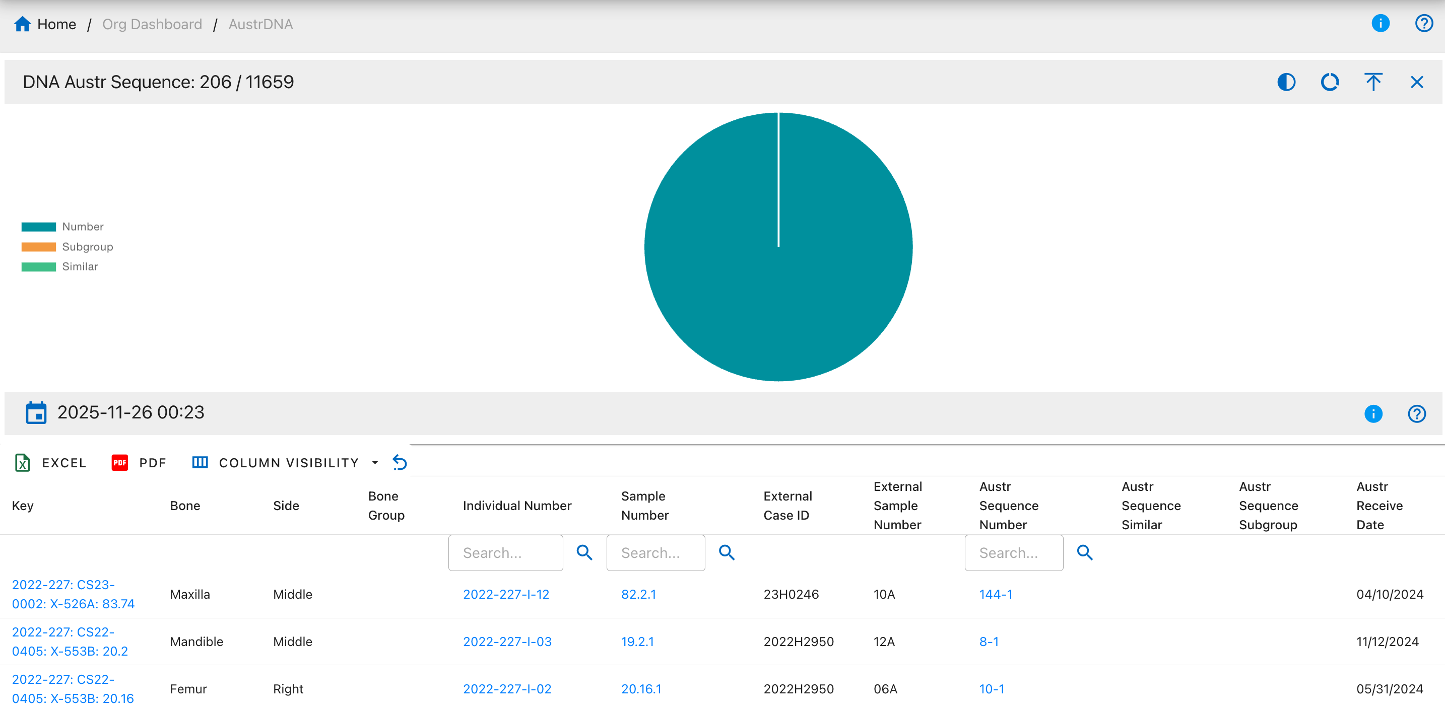
Pie Chart Segments:
- Number
- Subgroup
- Similar
DNA AuSTR Loci
The DNA AuSTR Loci drilldown displays samples with information about specific autosomal STR loci analyzed.

Pie Chart Segments:
- Loci Typed
- Loci Not Typed
DNA AuSTR MCC Dates
The DNA AuSTR MCC Dates drilldown shows samples with MCC-specific autosomal STR dates.

Pie Chart Segments:
- Reviewed
- Not Reviewed
Y-Chromosome STR (Y-STR) Drilldowns
Table Fields
- Key - Unique record identifier assigned to each DNA sample entry in the system for tracking and reference purposes
- Bone - Skeletal bone element name indicating the specific bone from which the DNA sample was collected (e.g., Femur, Humerus, Tibia)
- Side - Anatomical side designation showing whether the bone is from the Left or Right side of the body
- Bone Group - Bone classification category grouping similar bones together for organizational and analytical purposes (e.g., Long Bones, Skull, Ribs)
- Individual Number - Associated individual identifier linking the DNA sample to a specific person or skeletal remains for identification purposes
- Sample Number - DNA sample identifier serving as the primary unique reference number for the specific DNA sample collected
- External Case ID - External case reference number used by outside agencies or laboratories to track the case
- External Sample Number - External sample reference number assigned by external laboratories or agencies for their tracking purposes
- Y-STR Sequence Number - Y-chromosome STR sequence identifier representing the unique Y-STR profile assigned after analysis
- Y-STR Sequence Similar - Similar Y-chromosome STR sequences showing other samples that share matching or closely related profiles
- Y-STR Sequence Subgroup - Y-chromosome STR sequence subcategory providing additional classification detail within the main sequence group
- Y-STR Receive Date - Date Y-chromosome STR DNA results were received from the laboratory, marking when analysis was completed
DNA Y-STR Methods
The DNA Y-STR Methods drilldown shows DNA samples categorized by the method used for Y-chromosome STR analysis.
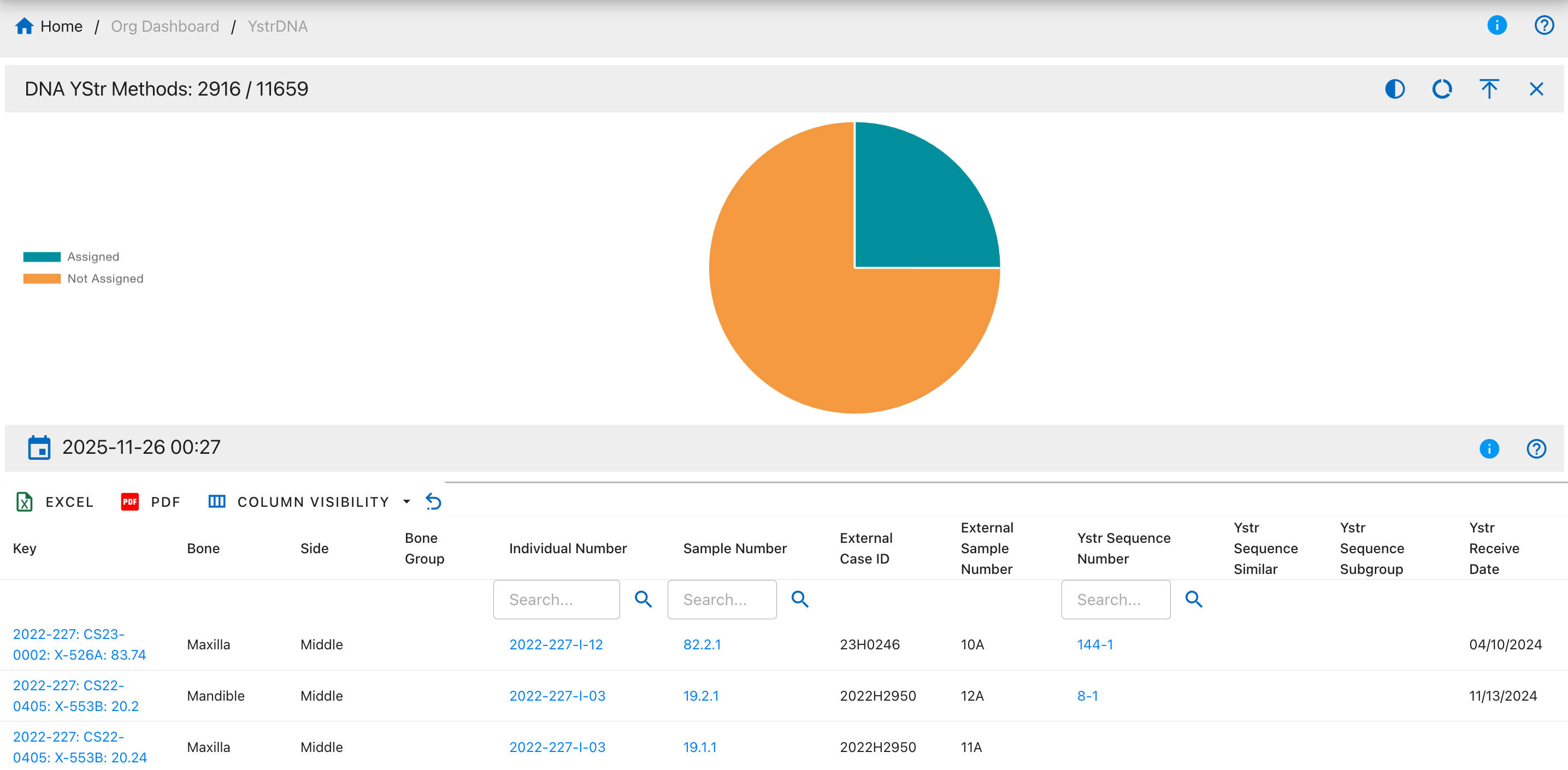
Pie Chart Segments:
- Assigned
- Not Assigned
DNA Y-STR Results
The DNA Y-STR Results drilldown displays all DNA samples with Y-chromosome short tandem repeat analysis results.
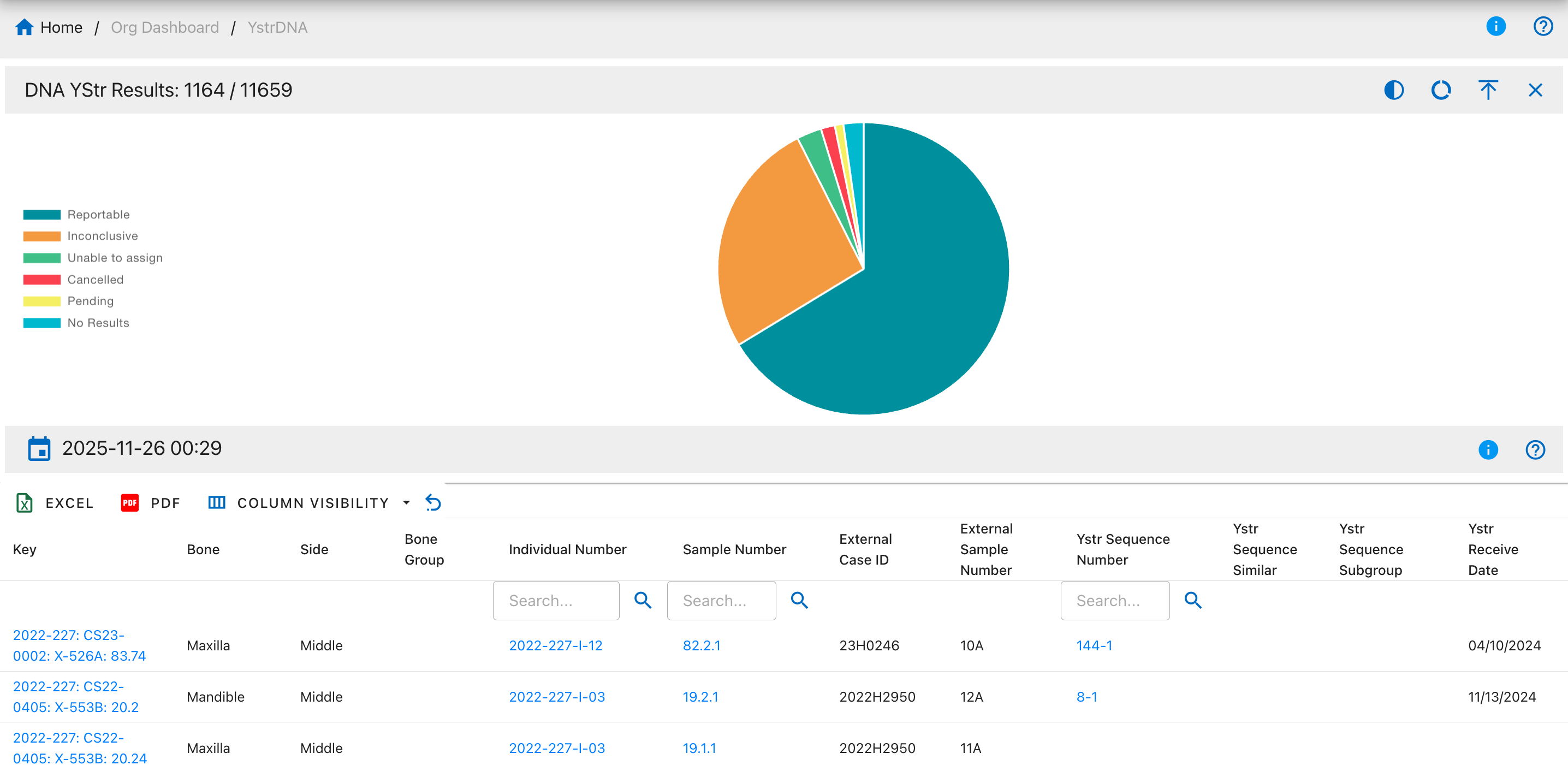
Pie Chart Segments:
- Reportable
- Inconclusive
- Unable to assign
- Cancelled
- Pending
- No Results
DNA Y-STR Dates
The DNA Y-STR Dates drilldown displays samples with Y-chromosome STR request and receive dates.
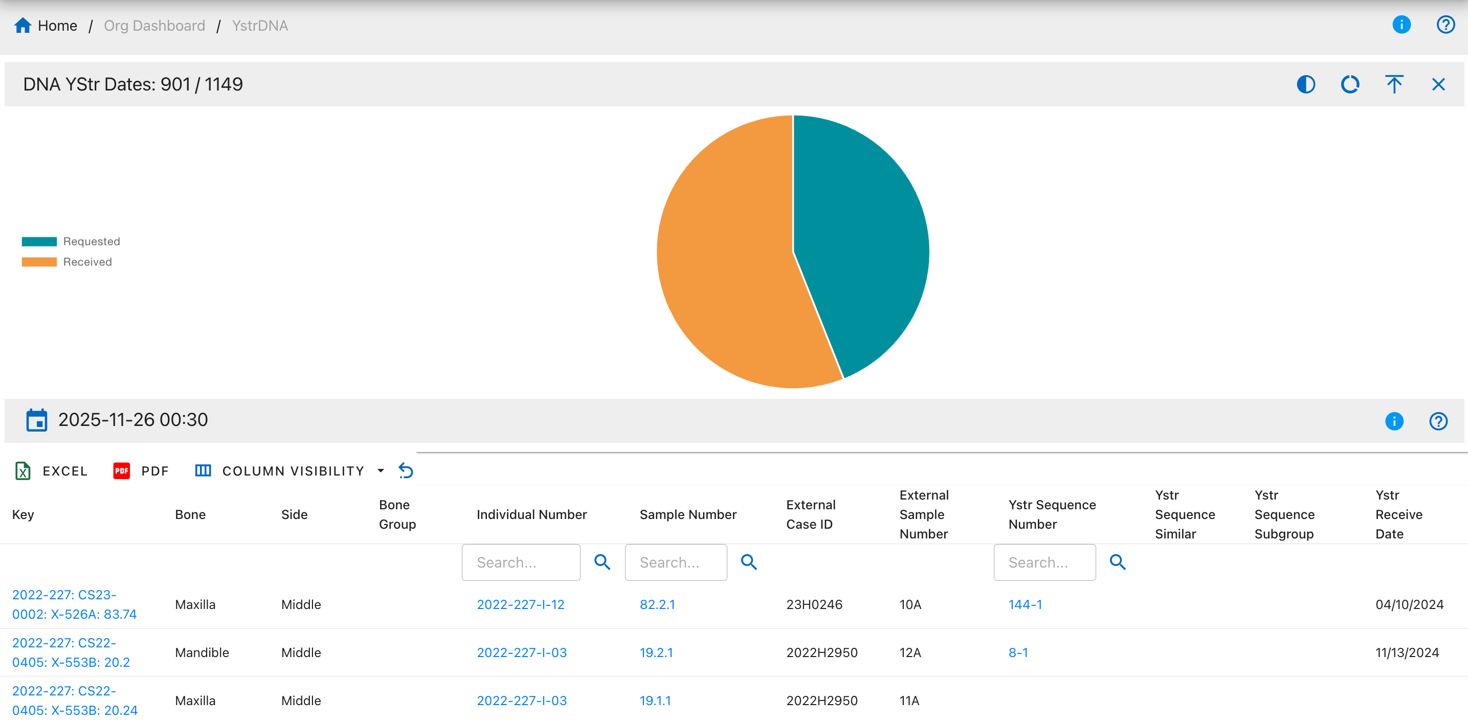
Pie Chart Segments:
- Requested
- Received
DNA Y-STR Sequence
The DNA Y-STR Sequence drilldown shows samples with assigned Y-chromosome STR sequence numbers.

Pie Chart Segments:
- Number
- Subgroup
- Similar
DNA Y-STR Loci
The DNA Y-STR Loci drilldown displays samples with information about Y-chromosome STR loci analyzed.

Pie Chart Segments:
- Loci Typed
- Loci Not Typed
DNA Y-STR Counts
The DNA Y-STR Counts drilldown shows Y-chromosome STR samples with match count data.

Pie Chart Segments:
- Match Count
- Total Count
DNA Y-STR MCC Dates
The DNA Y-STR MCC Dates drilldown displays samples with Y-STR MCC-specific dates.
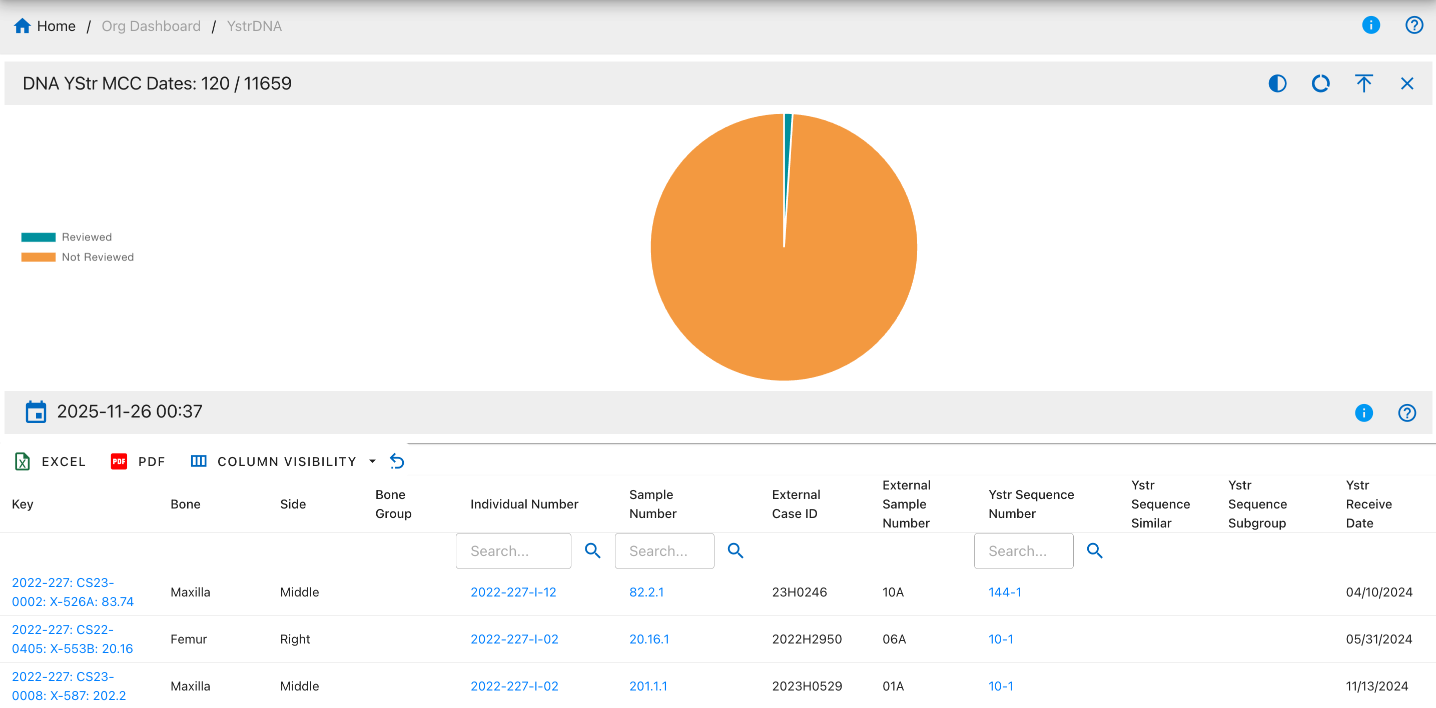
Pie Chart Segments:
- Reviewed
- Not Reviewed
Individual Dashboard Drilldowns
Warning
This page is work in progress.
The dashboard drilldown page provides information on the the drilldown charts and graphs from the dashboard.
Isotope Dashboard Drilldowns
This page documents the drilldown views available from the Isotope Dashboard. Each drilldown provides detailed tabular data corresponding to a specific isotope analysis metric or category. Users can search, filter, sort, and export data from these views.
Key Features
- Interactive Charts - Click any pie chart to view detailed sample data
- Advanced Search - Real-time filtering across all columns
- Data Export - Export to Excel or PDF with organization branding
- Clickable Links - Navigate directly to specimens, individuals, and bone groups
- Pagination - Server-side pagination for optimal performance
- Column Visibility - Toggle columns on/off and save preferences
- Multi-Sort - Sort by multiple columns simultaneously
How Drilldown Works
User Workflow
graph LR
    A[View Dashboard] --> B[Click Pie Chart]
    B --> C[New Tab Opens]
    C --> D[Large Chart Display]
    D --> E[Data Table Below]
    E --> F[Search/Filter/Export]
    F --> G[Click Sample Links]
    G --> H[View Details]
Navigation
Click on the detail button on any chart widget in the Isotope Dashboard to access its corresponding drilldown page. Each drilldown displays a visual representation of the data at the top, followed by a detailed data table below.
Available Actions
Search
Use the search bar at the top to find specific samples by entering text in the search field (e.g., sample number, bone name, individual number). The search is real-time and filters across all visible columns.
Real-Time Search
The search bar provides instant filtering across all visible columns:
- Case-Insensitive - Searches match regardless of capitalization
- Multi-Column - Searches across all text fields simultaneously
- Instant Results - Table updates as you type
- Clear Button - Quick reset to show all results
Search Examples
| Search Term | Matches | Use Case |
|---|---|---|
ISO-7 |
All samples from project 7 | Filter by project |
CIL 2003 |
Samples from CIL 2003 accession | Filter by accession |
Femur |
All femur samples | Filter by bone type |
Left |
All left-sided bones | Filter by side |
2025-123 |
Specific individual number | Find individual's samples |
Sort
Click any column header to sort data in ascending or descending order for easy data organization. Hold Shift and click multiple headers for multi-column sorting.
Single-Column Sort
- Click any column header to sort by that column
- First click: Ascending order (A→Z, 0→9)
- Second click: Descending order (Z→A, 9→0)
- Third click: Remove sort
Multi-Column Sort
- Click the first column header to set primary sort
- Hold Shift key while clicking additional column headers
- Sort priority follows click order
- Example: Sort by Bone (ascending), then Side (ascending)
Default Sort
- Default: Sorted by specimen Key (ascending)
- Format:
AccessionNumber:Provenance1:Provenance2:Designator - Purpose: Groups samples from same specimen together
Excel Export
Export the filtered isotope data to an Excel spreadsheet for advanced analysis, reporting, or data sharing. The export includes all visible columns and respects current filters and search terms.
Excel Export Features
- File Format:
.xlsxcompatible with Microsoft Excel and Google Sheets - Includes: All visible columns from current view
- Data Types: Preserves numbers, text, and dates properly
- Metadata: Organization and project information in header
- Filtering: Exports currently filtered/searched data only
- Use Cases:
- Advanced statistical analysis
- Lab reports and documentation
- Data sharing with collaborators
- Import into statistical software
Filename Format
Example:
PDF Export
Generate a printable PDF report of the isotope data with organization branding. The PDF includes headers, footers, and maintains the table structure for professional documentation.
PDF Export Features
- File Format: Professional PDF report with formatting
- Branding: Includes organization logo and header information
- Layout: Maintains column structure and alignment
- Page Numbers: Automatic page numbering and generation timestamp
- Print-Ready: Optimized for printing and archiving
- Filtering: Exports currently filtered/searched data only
- Use Cases:
- Quality control documentation
- Official lab reports
- Archival records
- Manuscript supplementary materials
- Regulatory compliance documentation
Filename Format
Example:
Column Visibility
Show or hide columns to customize your view by clicking the column visibility icon. Your preferences are saved automatically and persist across sessions.
Additional Actions
- Pagination - Navigate through large datasets using the pagination controls at the bottom of the table
- Items per Page - Adjust the number of rows displayed (10, 25, 50, 100) using the dropdown menu
- View Details - Click on any linked field (Key, Individual Number, Sample Number, Bone Group) to view complete details
- Refresh Data - Reload the table with the most current data by refreshing the browser
Table Fields
All isotope drilldowns display the following table columns:
- Key - Specimen identifier in format AN:P1:P2:Designator (Accession Number : Provenance1 : Provenance2 : Designator) serving as the unique specimen reference
- Bone - Skeletal bone element name indicating the specific bone from which the isotope sample was collected (e.g., Femur, Tibia, Humerus, Rib)
- Side - Anatomical side designation showing whether the bone is from the Left or Right side of the body, or if it is Middle/Unsided
- Bone Group - Bone classification category grouping similar bones together for organizational and analytical purposes
- Individual Number - Associated individual identifier linking the isotope sample to a specific person or skeletal remains for identification purposes
- Sample Number - Isotope sample identifier serving as the primary unique reference number for the specific isotope sample in format ISO-{project_id}-{number} (e.g., ISO-7-000001)
Isotope Analysis Drilldowns
Isotope Results
The Isotope Results drilldown displays all isotope samples that have assigned results confidence levels recorded. This view helps track the quality and reliability of isotope analysis results across samples.
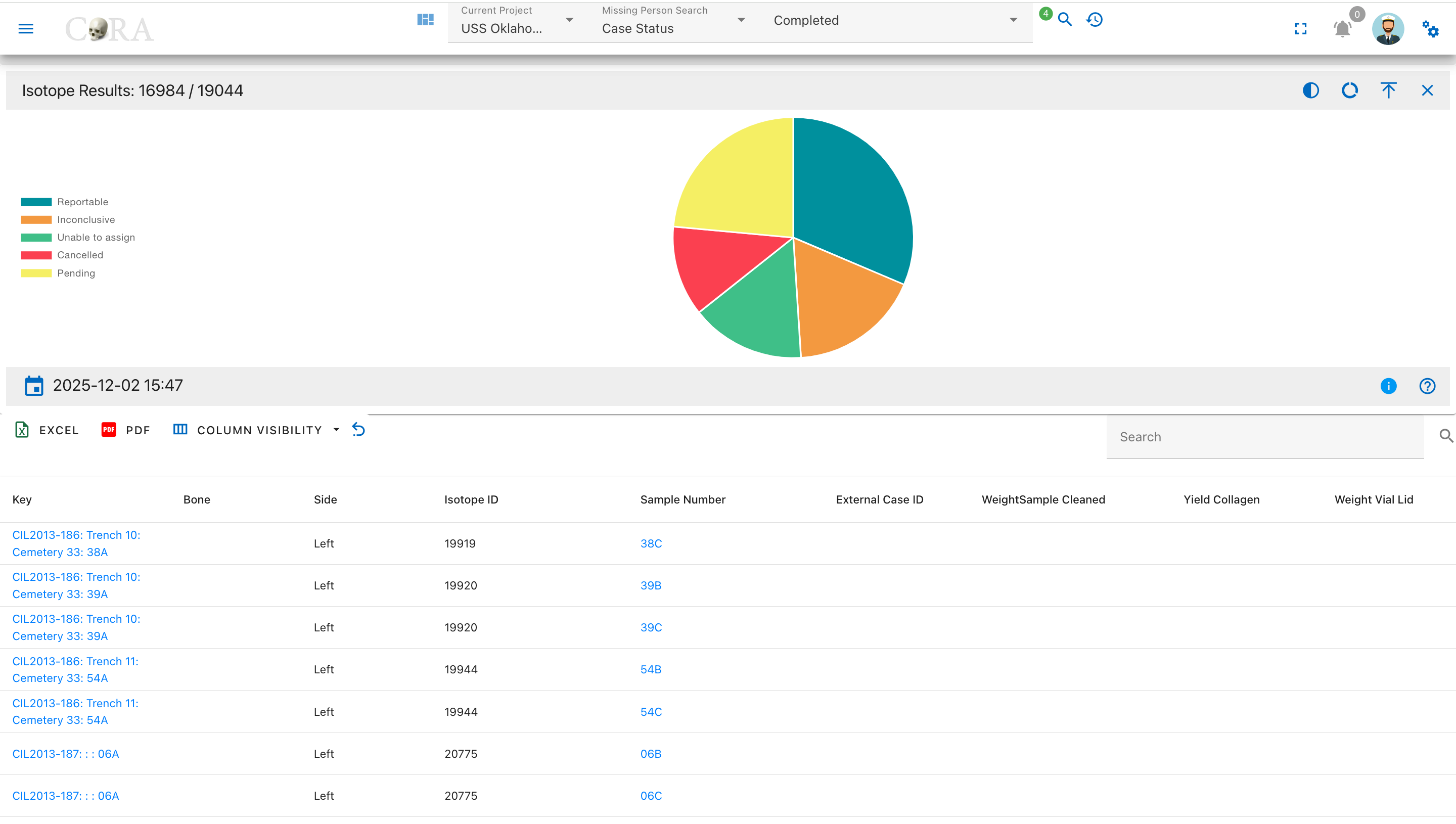
Pie Chart Segments:
- Reportable
- Inconclusive
- Unable to Assign
- Cancelled
- Pending
Results Status
The Results Status drilldown shows the overall reporting status of isotope samples, indicating which samples have completed analysis with reportable results.
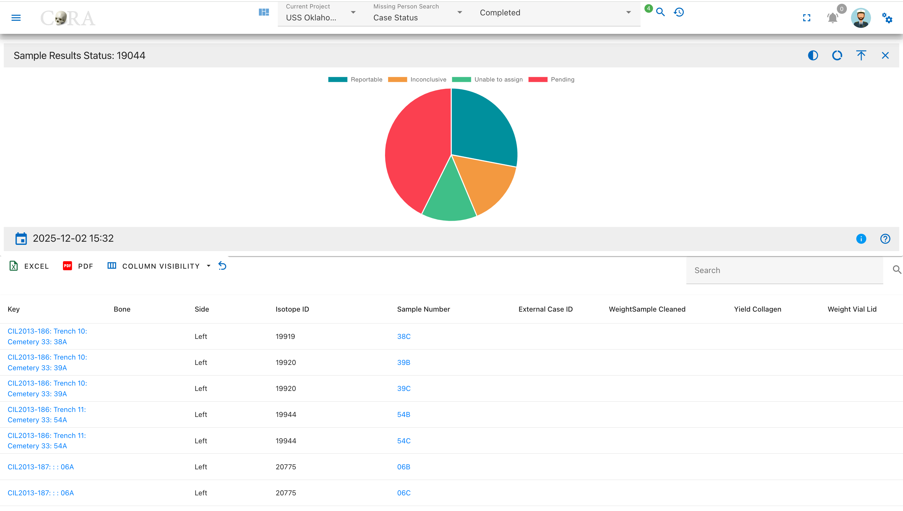
Pie Chart Segments:
- Reportable
- Inconclusive
- Unable to Assign
- Pending
Collagen Processing Drilldowns
Collagen Weights
The Collagen Weights drilldown displays samples with recorded collagen weight used for isotope analysis, showing the amount of extracted collagen available.
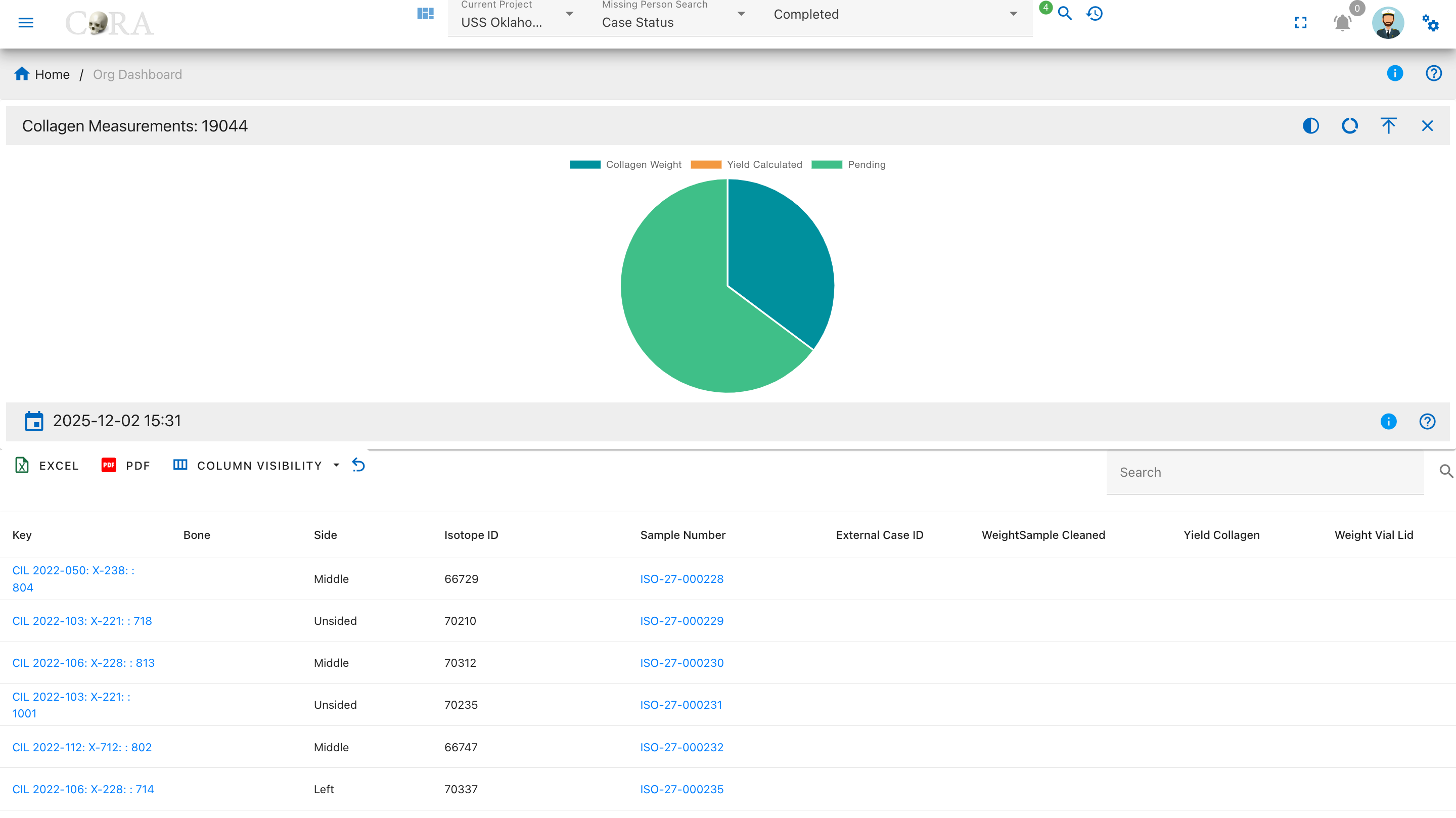
Pie Chart Segments:
- Collagen Weight Recorded
- Pending
Weight Measurement Drilldowns
Vial Weights
The Vial Weights drilldown displays samples with recorded vial and lid weights, which are necessary for calculating net sample weights.
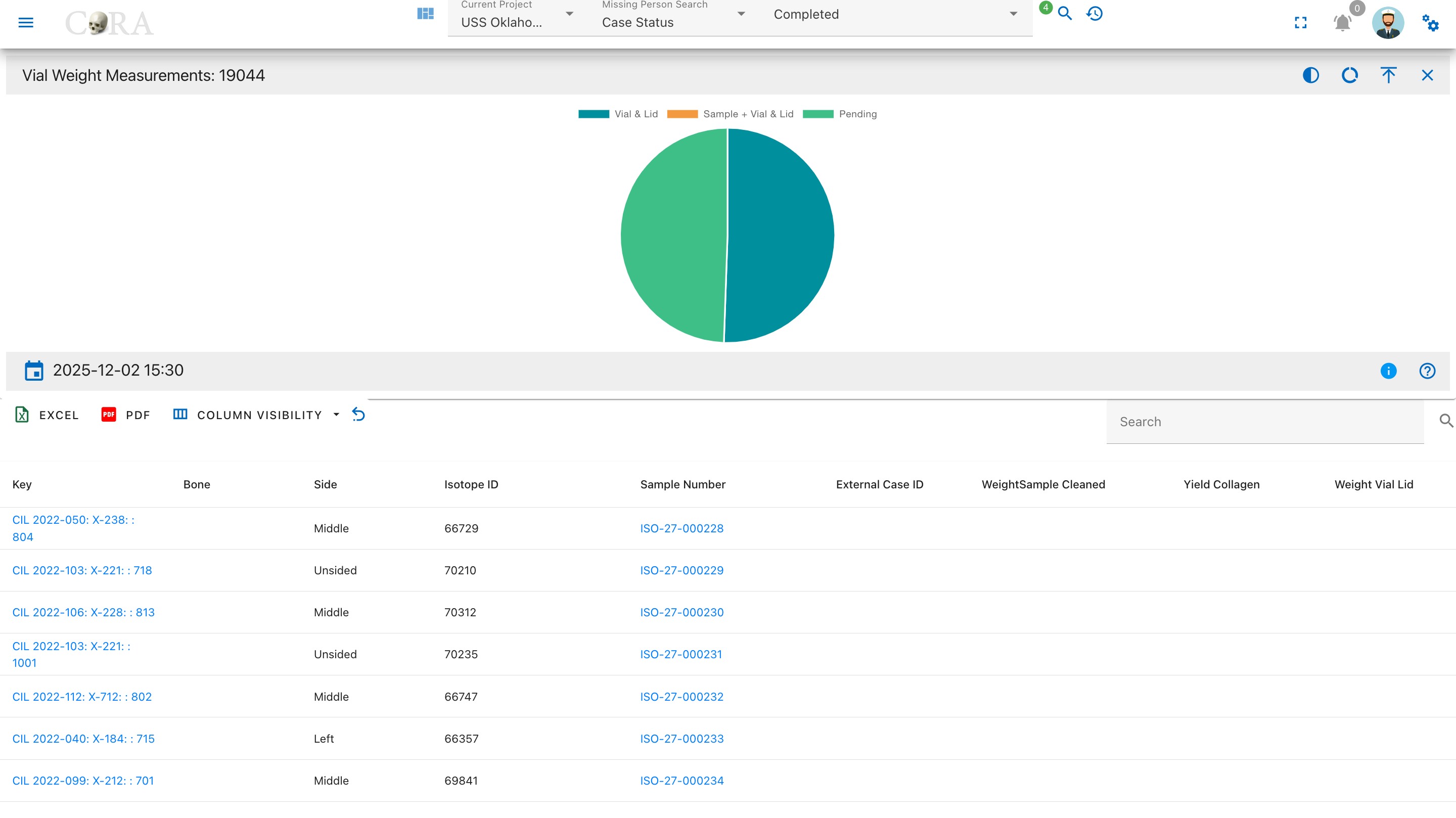
Pie Chart Segments:
- Vial & Lid Weighed
- Pending
Weight Status
The Weight Status drilldown shows samples categorized by whether any weight measurements have been recorded across all weight fields.
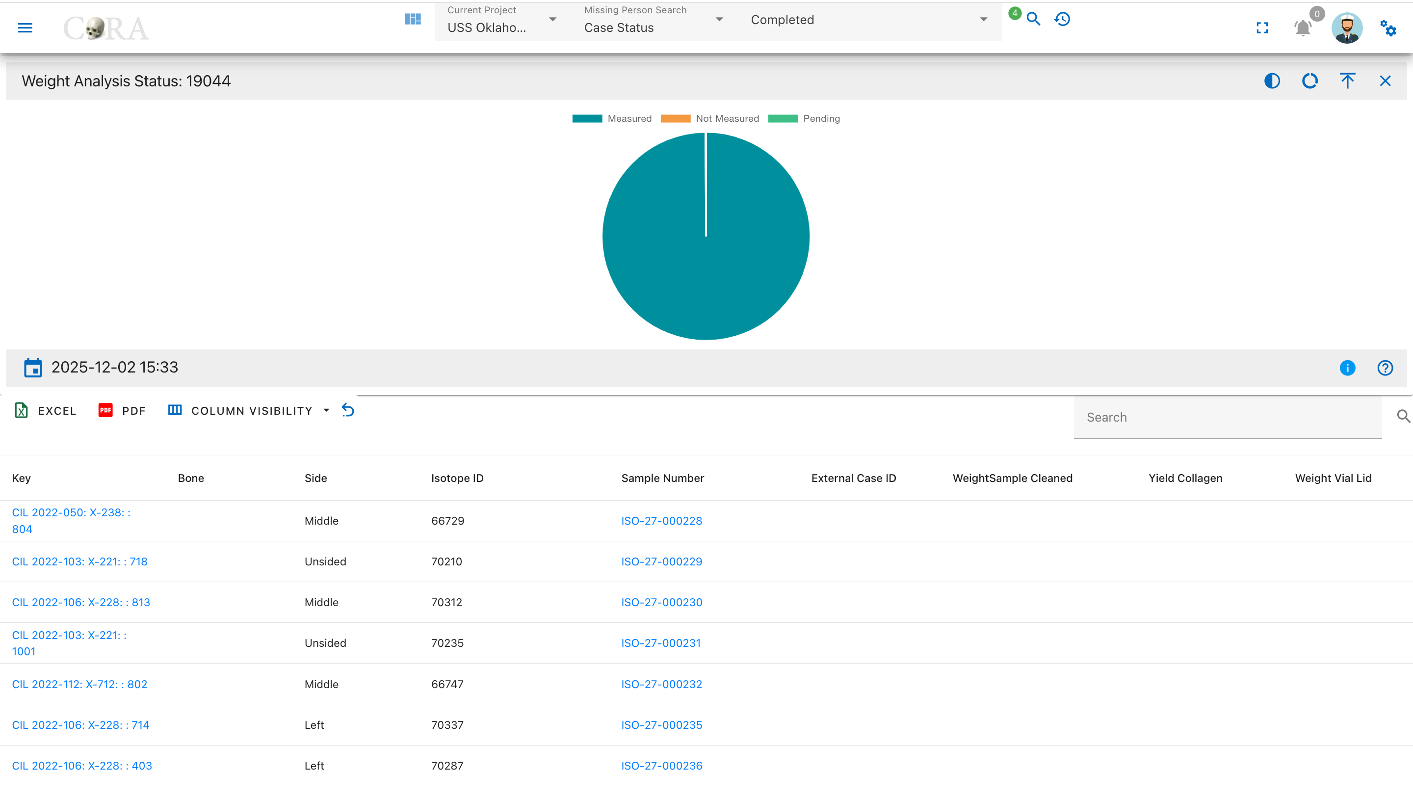
Pie Chart Segments:
- Measured
- Not Measured
- Pending
Demineralization Processing Drilldowns
Demineralization Status
The Demineralization Status drilldown displays isotope samples categorized by their demineralization processing status, showing which samples have started and completed this critical preparation step.
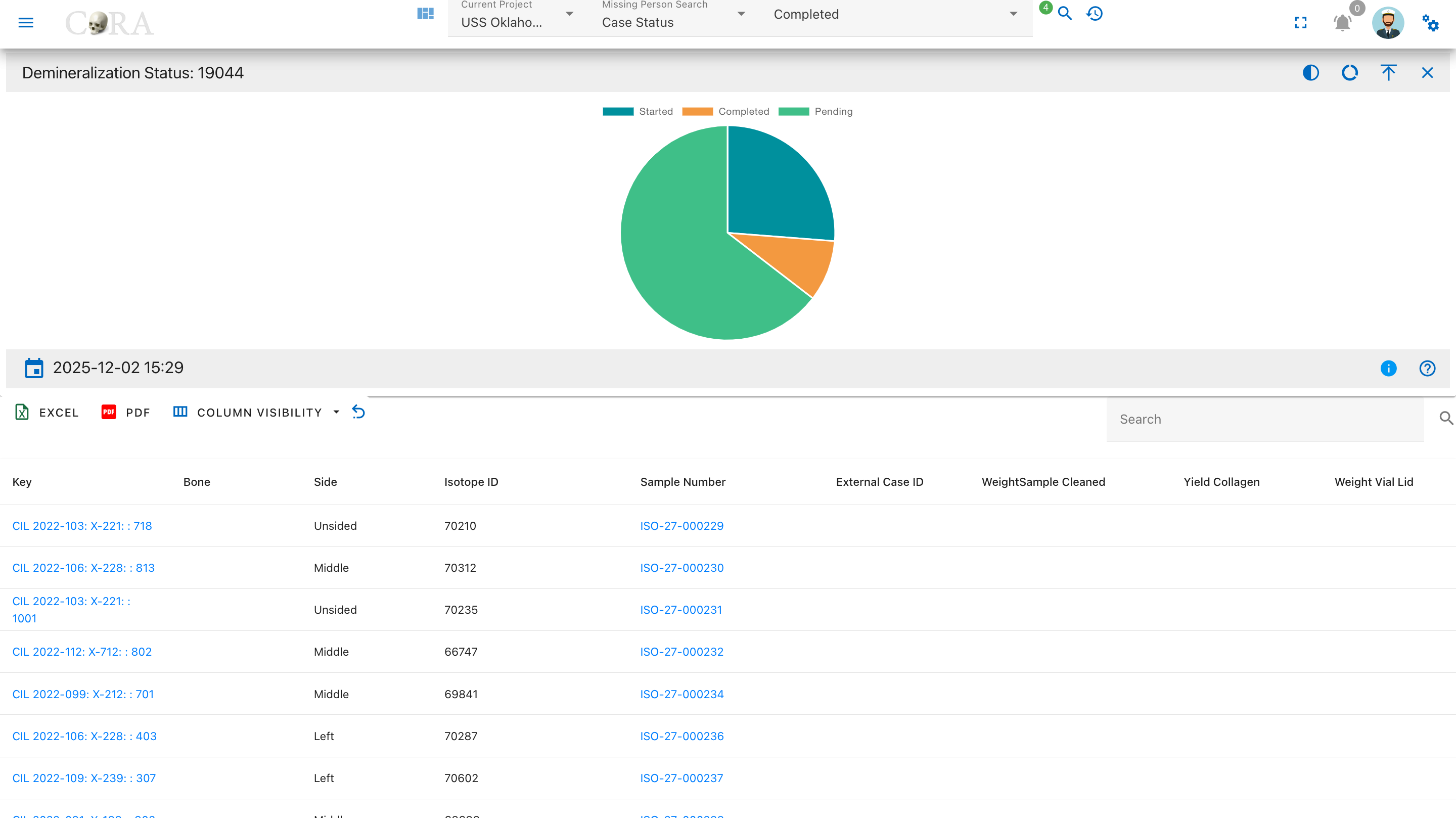
Pie Chart Segments:
- Started
- Completed
- Pending
Isotope Ratio Drilldowns
Carbon to Nitrogen (C:N) Ratio
The C:N Ratio drilldown displays samples categorized by their carbon to nitrogen ratio values, which indicate collagen preservation quality and sample integrity.
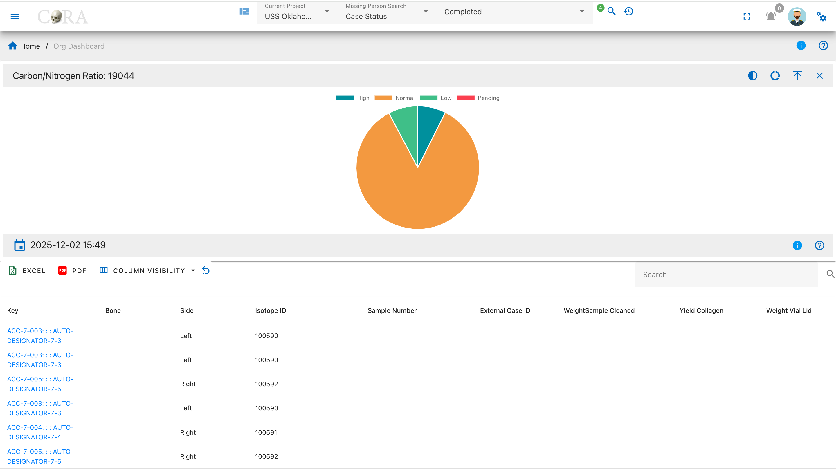
Pie Chart Segments:
- High (>3.6)
- Normal (2.9-3.6)
- Low (<2.9)
- Pending
Carbon to Oxygen (C:O) Ratio
The C:O Ratio drilldown shows samples categorized by their carbon to oxygen ratio, an indicator of isotopic stability and sample quality.
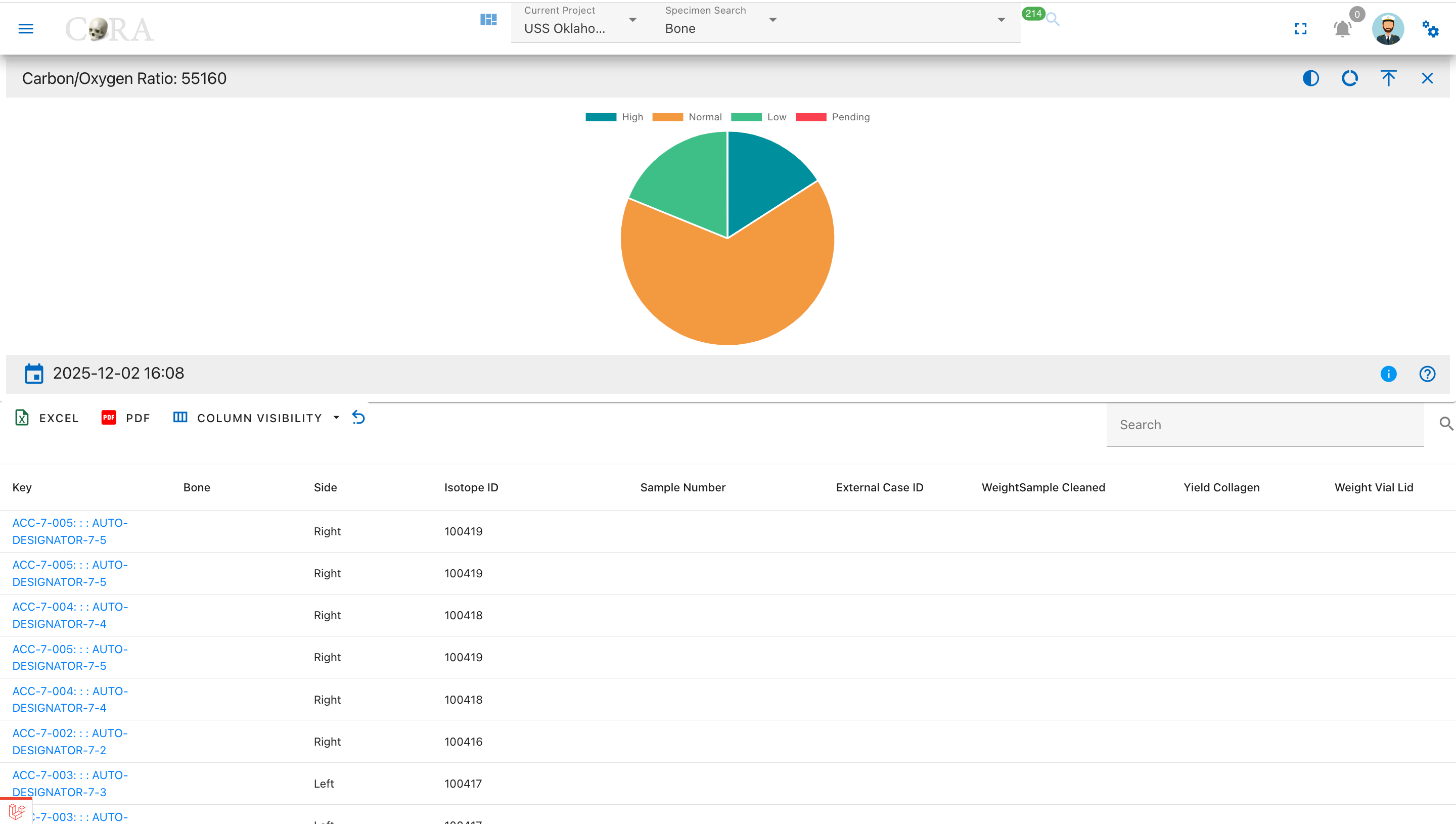
Pie Chart Segments:
- High (>1.4)
- Normal (1.1-1.4)
- Low (<1.1)
- Pending
Elemental Analysis Drilldowns
Carbon Analysis (δ¹³C)
The Carbon Analysis drilldown displays samples with carbon isotope measurements, showing delta values, weights, and percentages for carbon content.
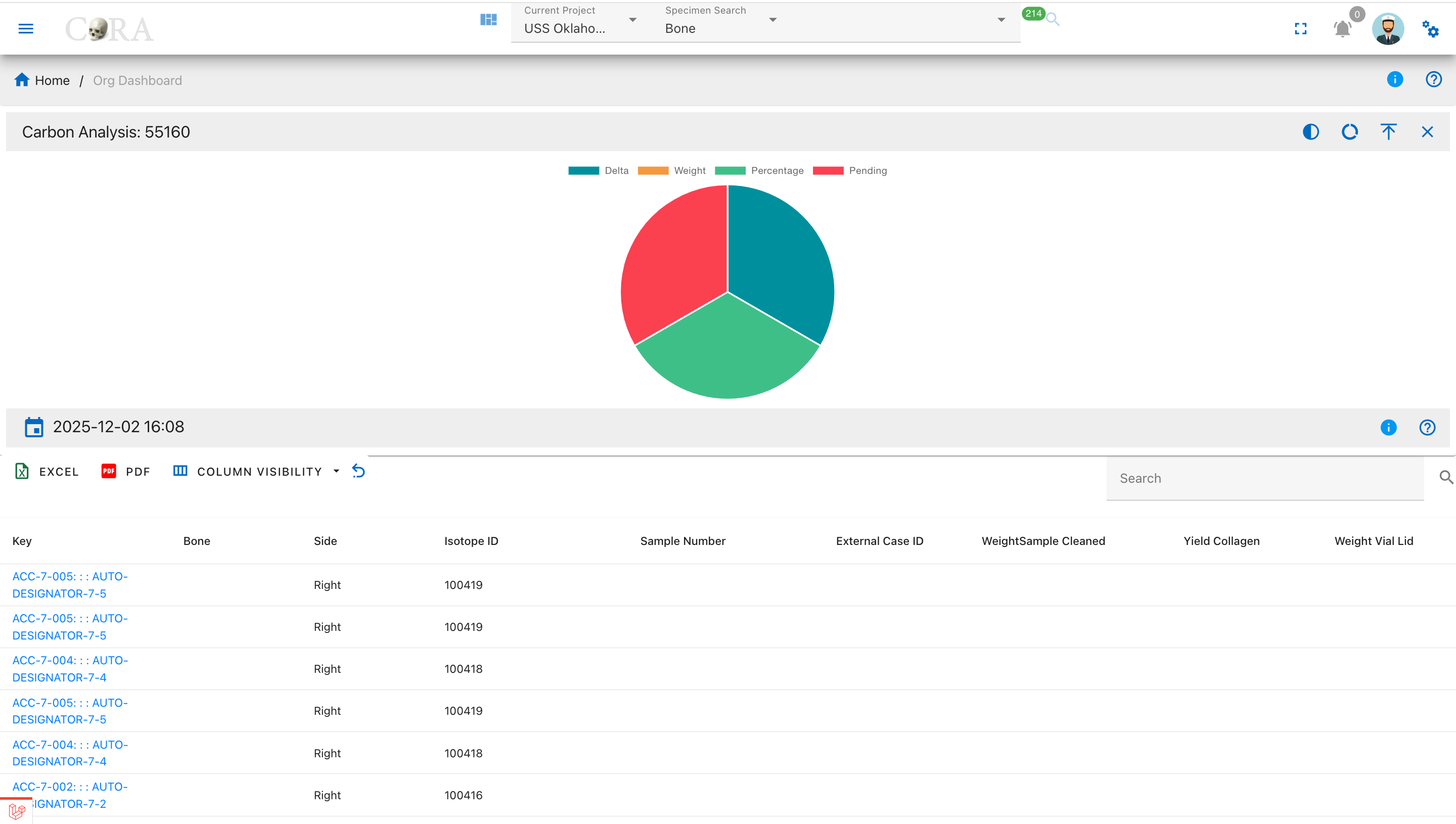
Pie Chart Segments:
- Delta (δ¹³C)
- Weight
- Percentage
- Pending
Nitrogen Analysis (δ¹⁵N)
The Nitrogen Analysis drilldown shows samples with nitrogen isotope measurements, displaying delta values, weights, and percentages for nitrogen content.
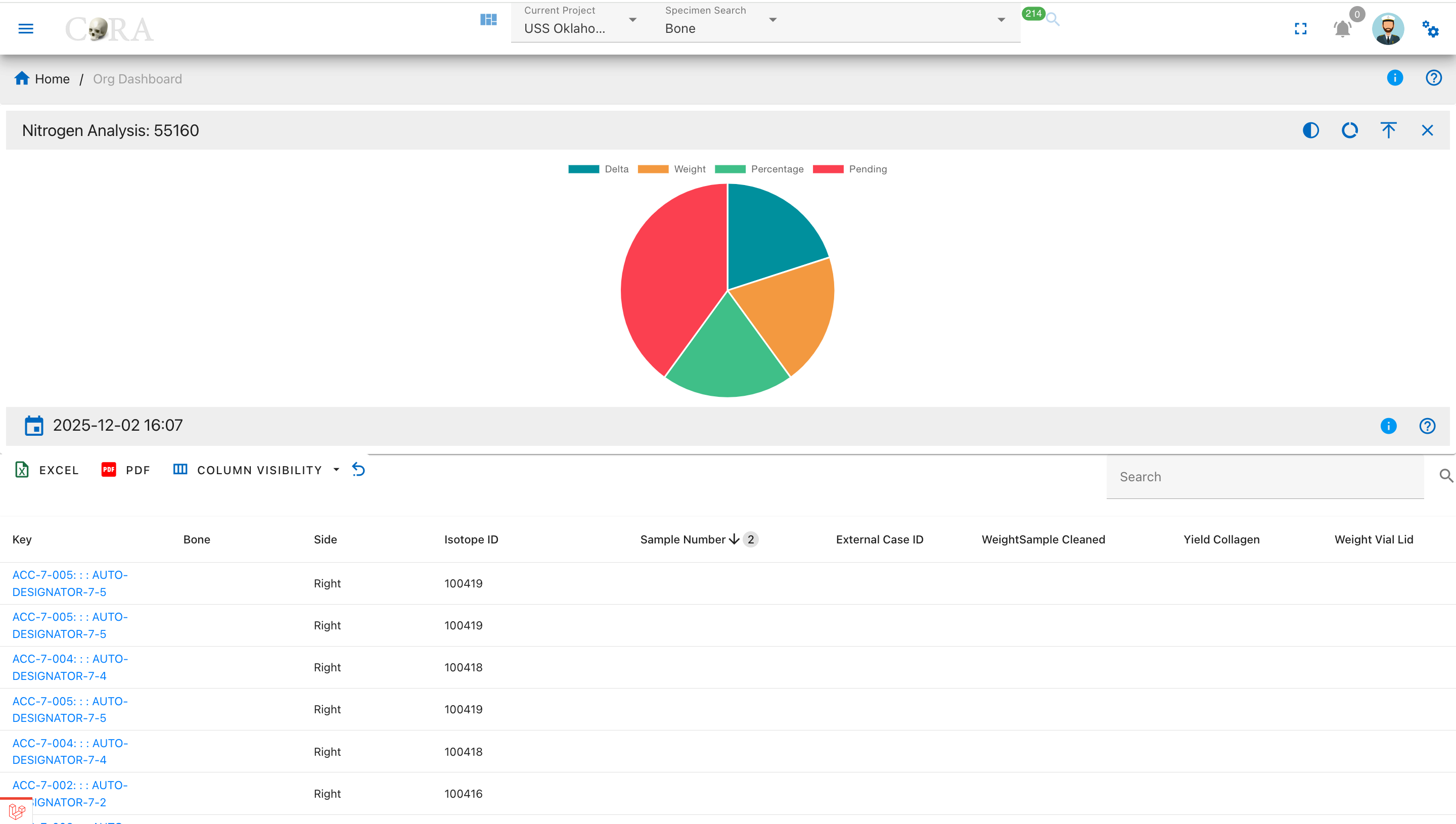
Pie Chart Segments:
- Delta (δ¹⁵N)
- Weight
- Percentage
- Pending
Oxygen Analysis (δ¹⁸O)
The Oxygen Analysis drilldown displays samples with oxygen isotope measurements, showing delta values, weights, and percentages for oxygen content.
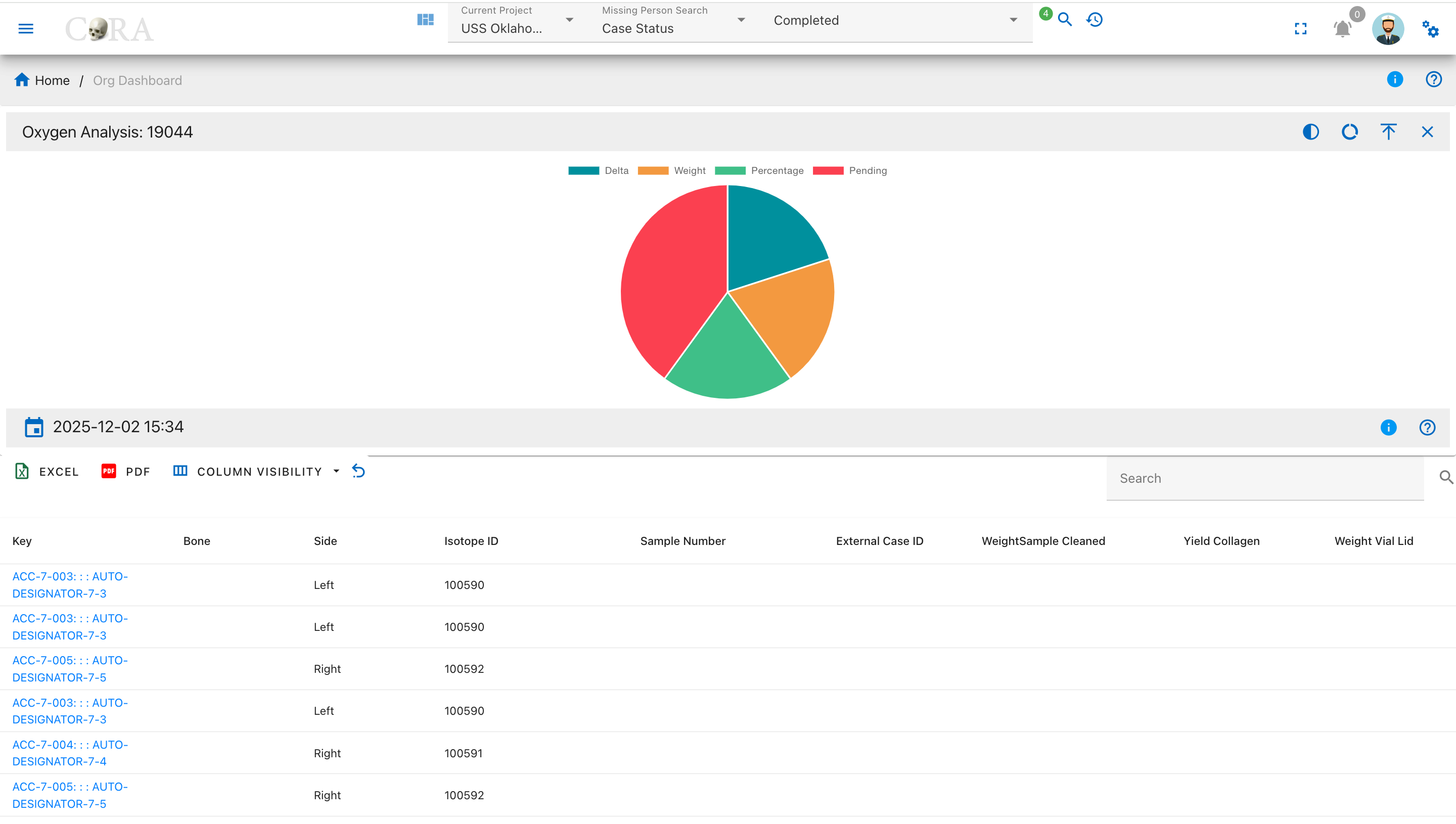
Pie Chart Segments:
- Delta (δ¹⁸O)
- Weight
- Percentage
- Pending
Sulphur Analysis (δ³⁴S)
The Sulphur Analysis drilldown shows samples with sulphur isotope measurements, displaying delta values, weights, and percentages for sulphur content.
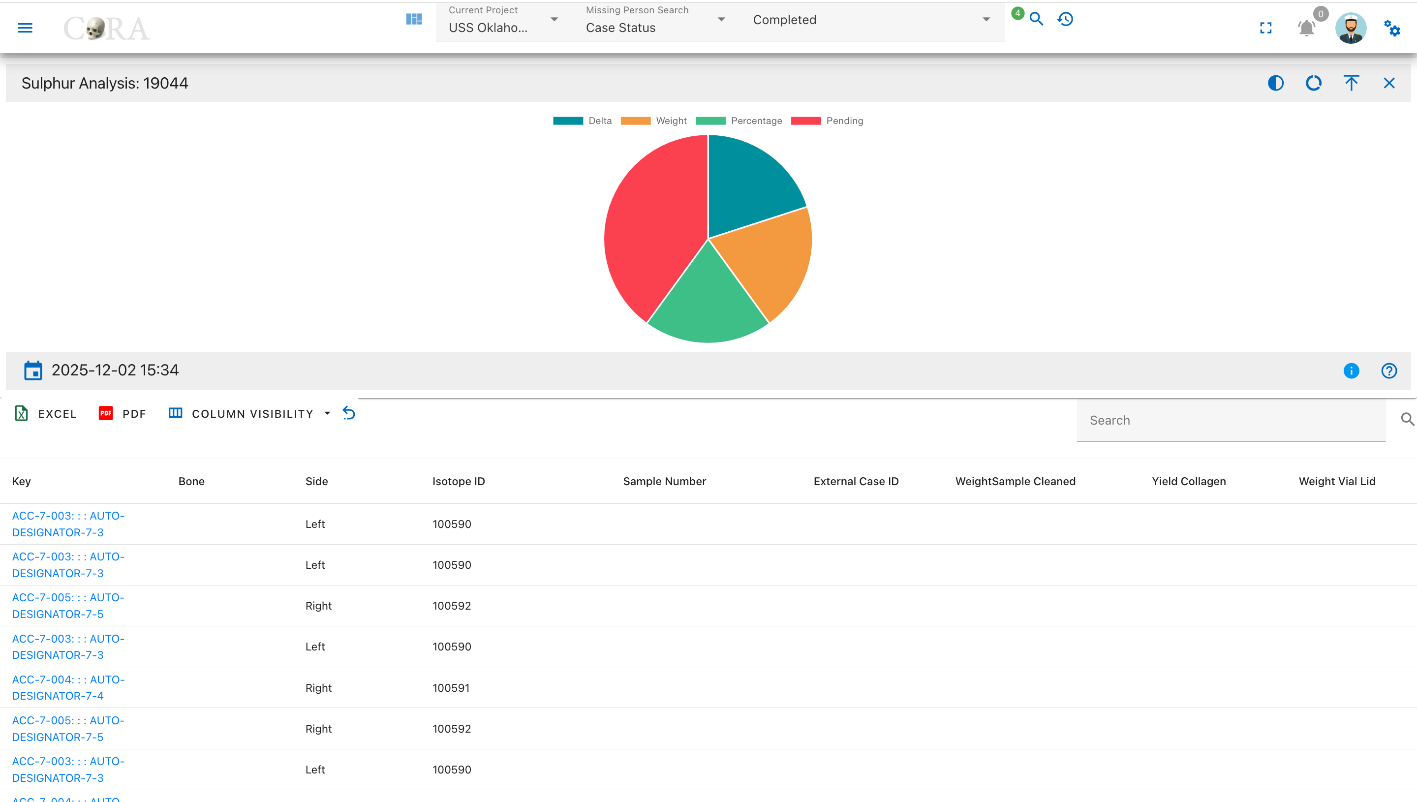
Pie Chart Segments:
- Delta (δ³⁴S)
- Weight
- Percentage
- Pending
Missing Person Dashboard Drilldowns
This section of the user guide describes the drilldown pages available from each widget on the Missing Person Dashboard. Each drilldown page provides an in-depth view of the selected data, featuring an interactive chart and a detailed, filterable table. These drilldowns help users investigate specific case details, apply advanced searches, and export results for further review.
The following pages explain what each drilldown displays, the meaning of each data field, and the actions users can perform, such as searching, filtering, sorting, and exporting.
Navigation
To access the drilldowns, click on the desired widget's chart segment in the main Missing Person Dashboard.
Table Fields
All drilldown data tables include these columns unless specifically noted:
- Case Number: Unique identifier for each case.
- Owner Service: Branch or agency responsible.
- Service Member Service: Affiliation of the missing individual.
- Case Status: Overall status.
- Full Name: Name of the missing person.
- Conflict: Associated conflict or mission.
- Incident: Incident details, if available.
- Case Manager: Assigned staff member.
- Project: Related project.
- Priority DPAA: DPAA project priority.
- Priority PCRB: PCRB project priority.
- DPAA Case Status: Status per DPAA records.
- Followed Up: Whether follow-up has been performed.
- Updated DCIP: Indicates if DCIP record is current.
- Genealogy Status: Status of genealogy research.
- Action: Edit or delete records, as permitted.
Exceptions:
- Case Managers Drilldown: Columns are Case Manager and Total only.
User Actions
All drilldown tables support:
- Searching and Filtering: Use search boxes under each column header.
- Sorting: Click any column header to sort the data.
- Export: Download data as Excel or PDF.
- Column Visibility: Show/hide columns with the dropdown.
- Refresh: Reload table data with the refresh icon.
- Record Management: Edit or delete records with action icons (where permitted).
Exceptions:
- Case Managers Drilldown: Only supports a single top-row search box, sorting, export, column visibility, and refresh. (No per-column filtering or record management.)
Drilldown Pages
For each drilldown below, refer to Table Fields and User Actions above for details on available columns and controls except where exceptions are listed.
Case Status
This page presents a detailed drilldown view of the Case Status widget from the Missing Person Dashboard. Users can analyze the status distribution of all missing person cases via an interactive pie chart and a comprehensive data table.
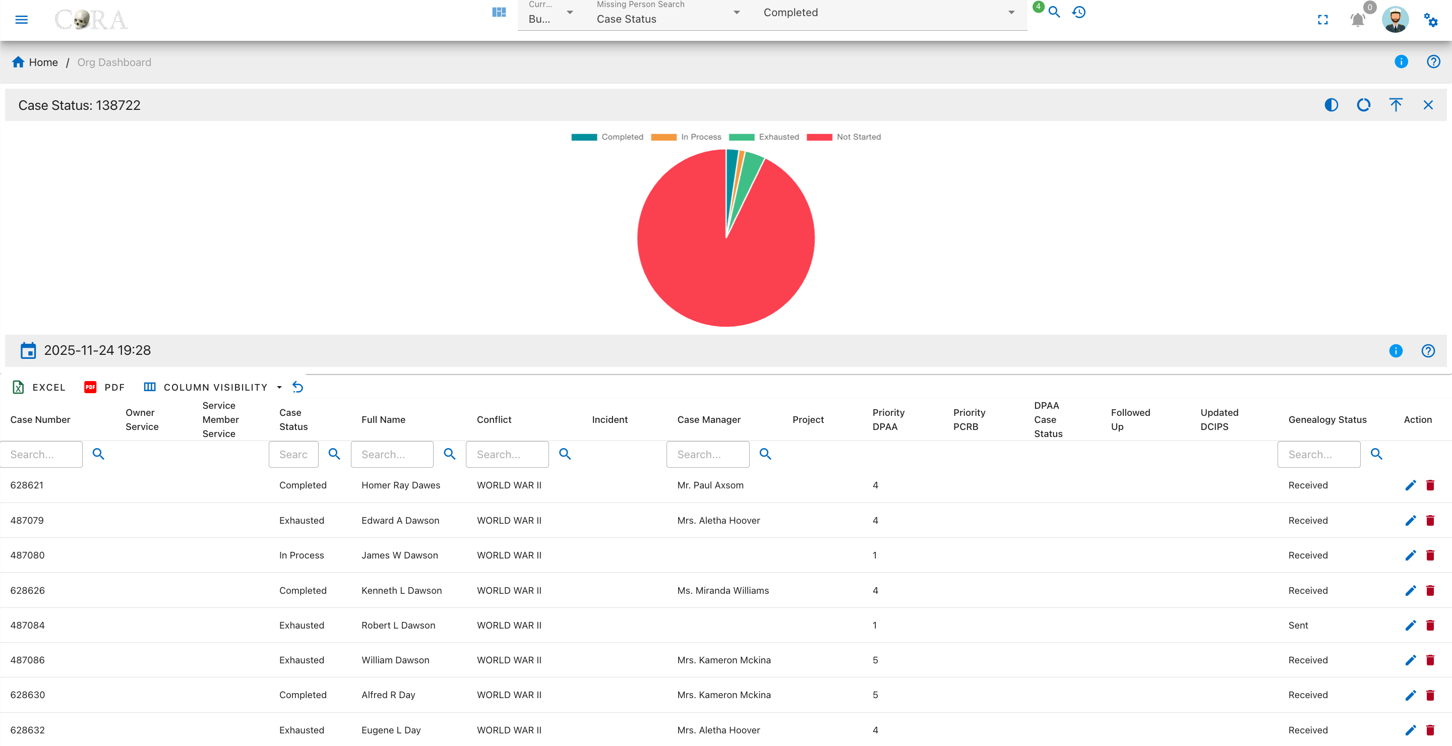
Overview
A pie chart on this page visualizes the case status distribution for all missing person records. The four status categories are:
- Completed
- In Process
- Exhausted
- Not Started
The chart legend defines each case status, and tooltips display the number of cases within each segment.
Genealogy Status
This page presents a detailed drilldown view of the Genealogy Status widget from the Missing Person Dashboard. Users can review the genealogy request progress for each missing person case, visualized by status in an interactive pie chart and detailed cases in a searchable table.
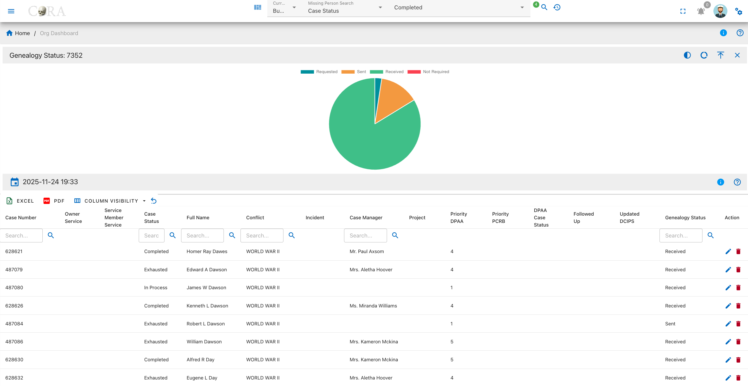
Overview
A pie chart on this page displays the breakdown of genealogy research statuses. The common categories include:
- Requested
- Sent
- Received
- Not Required
Hovering over the chart segments reveals the exact count for each category as shown in the legend.
FRS 1 MTDNA Status
This page displays a detailed drilldown of the FRS 1 MTDNA Status widget from the Missing Person Dashboard. Users can examine the statuses of Family Reference Sample (FRS) MTDNA requests for missing person cases, with both an interactive pie chart and a comprehensive data table.
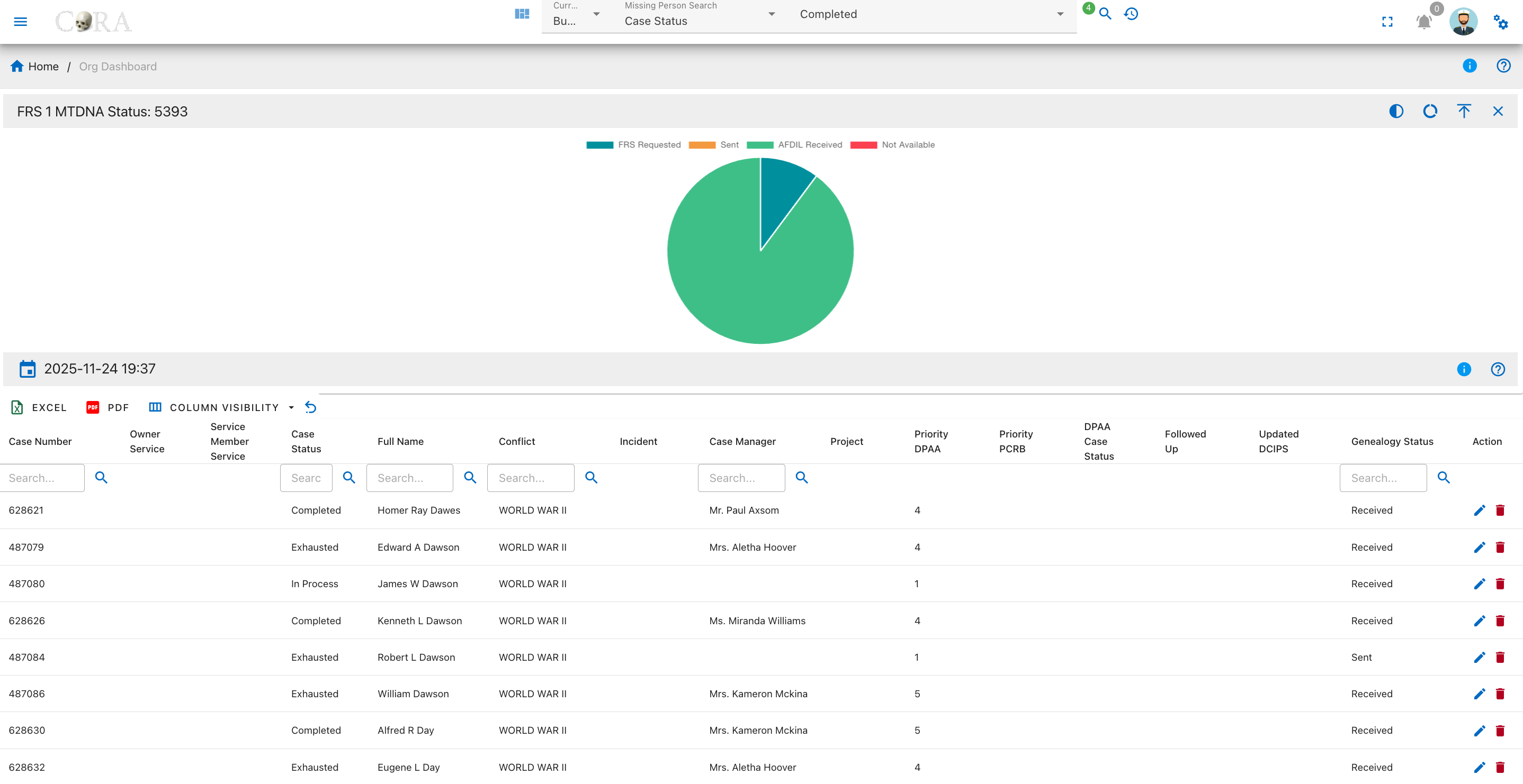
Overview
A pie chart on this page visualizes the current statuses for FRS 1 MTDNA requests. The four status categories are:
- FRS Requested
- Sent
- AFDIL Received
- Not Available
The chart legend identifies each status, and tooltips show precise case counts on hover.
FRS 2 MTDNA Status
This page presents a detailed drilldown view of the FRS 2 MTDNA Status widget from the Missing Person Dashboard. Users can review the fulfillment status for second Family Reference Sample (MTDNA) requests, visualized in an interactive pie chart and summarized in a comprehensive data table.
Overview
A pie chart on this page visualizes the current statuses for FRS 2 MTDNA requests. The four status categories are:
- FRS Requested
- Sent
- AFDIL Received
- Not Available
The chart legend identifies each status, and tooltips show precise case counts on hover.
FRS 3 MTDNA Status
This page presents a detailed drilldown view of the FRS 3 MTDNA Status widget from the Missing Person Dashboard. Users can review the status breakdown for third Family Reference Sample (MTDNA) requests across all missing person cases via an interactive pie chart and a searchable, filterable data table.
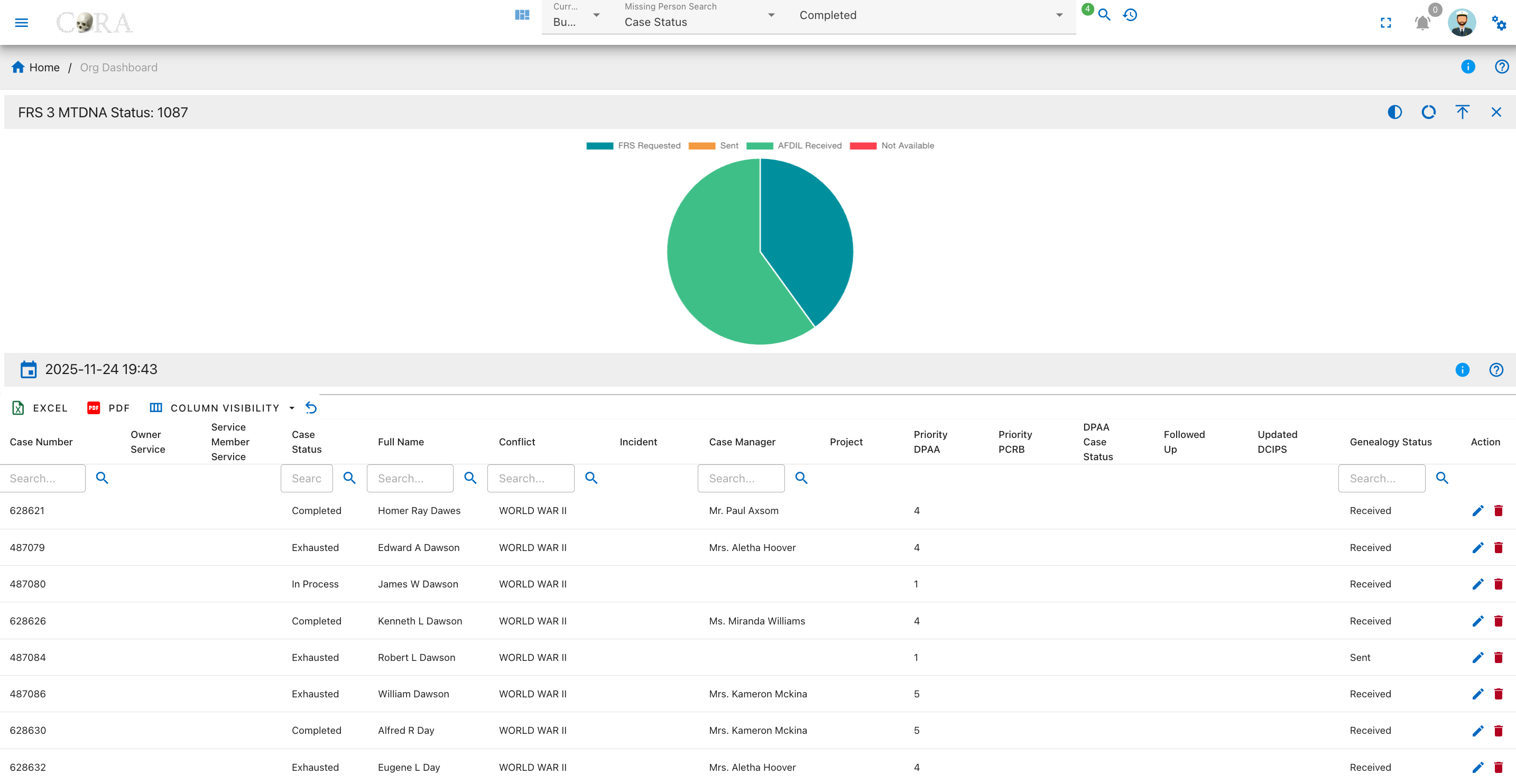
Overview
A pie chart on this page visualizes the current statuses for FRS 3 MTDNA requests. The four status categories are:
- FRS Requested
- Sent
- AFDIL Received
- Not Available
The chart legend identifies each status, and tooltips show precise case counts on hover.
FRS 1 YStr Status
This page presents a detailed drilldown view of the FRS 1 YStr Status widget from the Missing Person Dashboard. Users can analyze the progress and breakdown of first Family Reference Sample (YStr) requests for missing person cases, with both an interactive pie chart and a comprehensive data table.
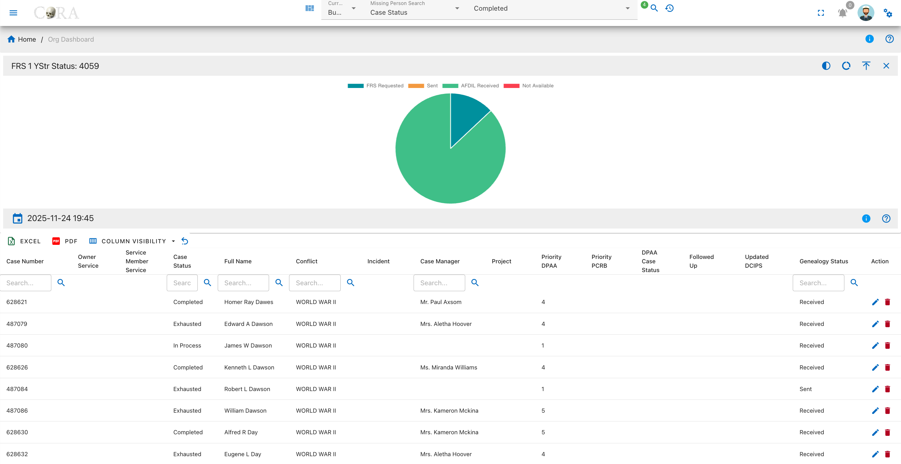
Overview
A pie chart on this page visualizes the status distribution for FRS 1 YStr sample requests. The four status categories are:
- FRS Requested
- Sent
- AFDIL Received
- Not Available
The legend defines each status; tooltips show how many cases fall into each group.
FRS 2 YStr Status
This page provides a breakdown of the second Family Reference Sample (YStr) request statuses for all missing person cases on the dashboard. Users can quickly visualize the distribution of FRS 2 YStr requests using an interactive pie chart and review detailed case information in a searchable, filterable data table.
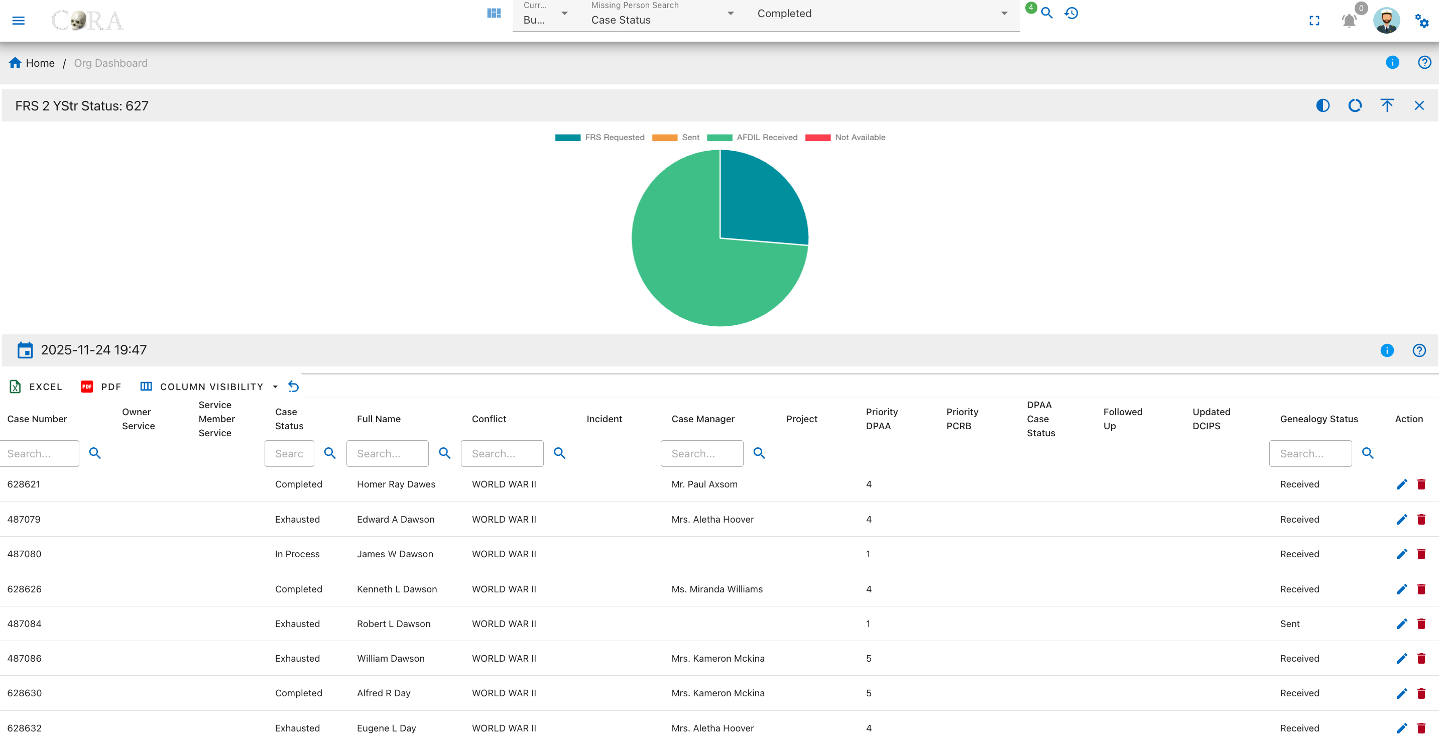
Overview
A pie chart on this page visualizes the status distribution for FRS 1 YStr sample requests. The four status categories are:
- FRS Requested
- Sent
- AFDIL Received
- Not Available
The legend defines each status; tooltips show how many cases fall into each group.
FRS 1 AUSTR Status
This page provides a detailed view of the first Family Reference Sample (AUSTR) request statuses for all missing person cases. The drilldown uses an interactive pie chart to visualize the distribution of AUSTR requests by status, alongside a searchable, filterable data table containing in-depth case data.
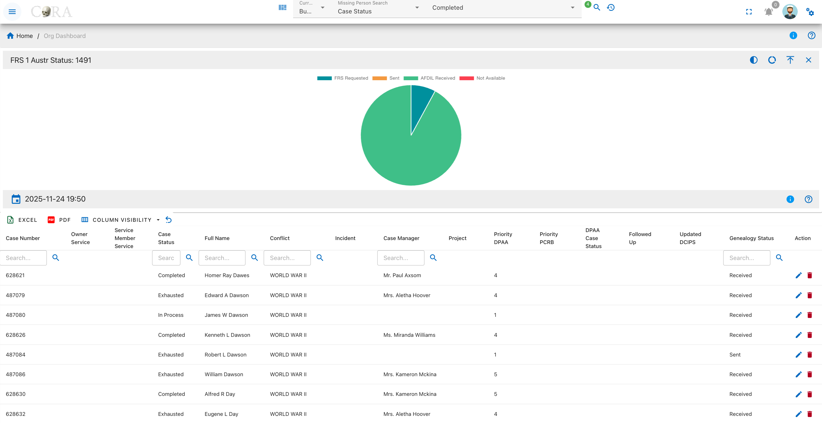
Overview
A pie chart on this page shows the breakdown of FRS 1 AUSTR request statuses. The primary categories are:
- FRS Requested
- Sent
- AFDIL Received
- Not Available
Each segment is labeled in the legend, and tooltips explain the case count for that status.
FRS 2 AUSTR Status
This page provides a detailed view of the second Family Reference Sample (AUSTR) request statuses for all missing person cases. The drilldown page features an interactive pie chart that visualizes the status distribution for FRS 2 AUSTR requests, as well as a searchable and filterable data table for in-depth case review.

Overview
A pie chart on this page shows the breakdown of FRS 2 AUSTR request statuses. The primary categories are:
- FRS Requested
- Sent
- AFDIL Received
- Not Available
Each segment is labeled in the legend, and tooltips explain the case count for that status.
Followed Up
This page provides a status summary of follow-up actions for missing person cases. The drilldown features an interactive pie chart and a detailed table, allowing users to quickly assess which cases have been followed up and which have not.
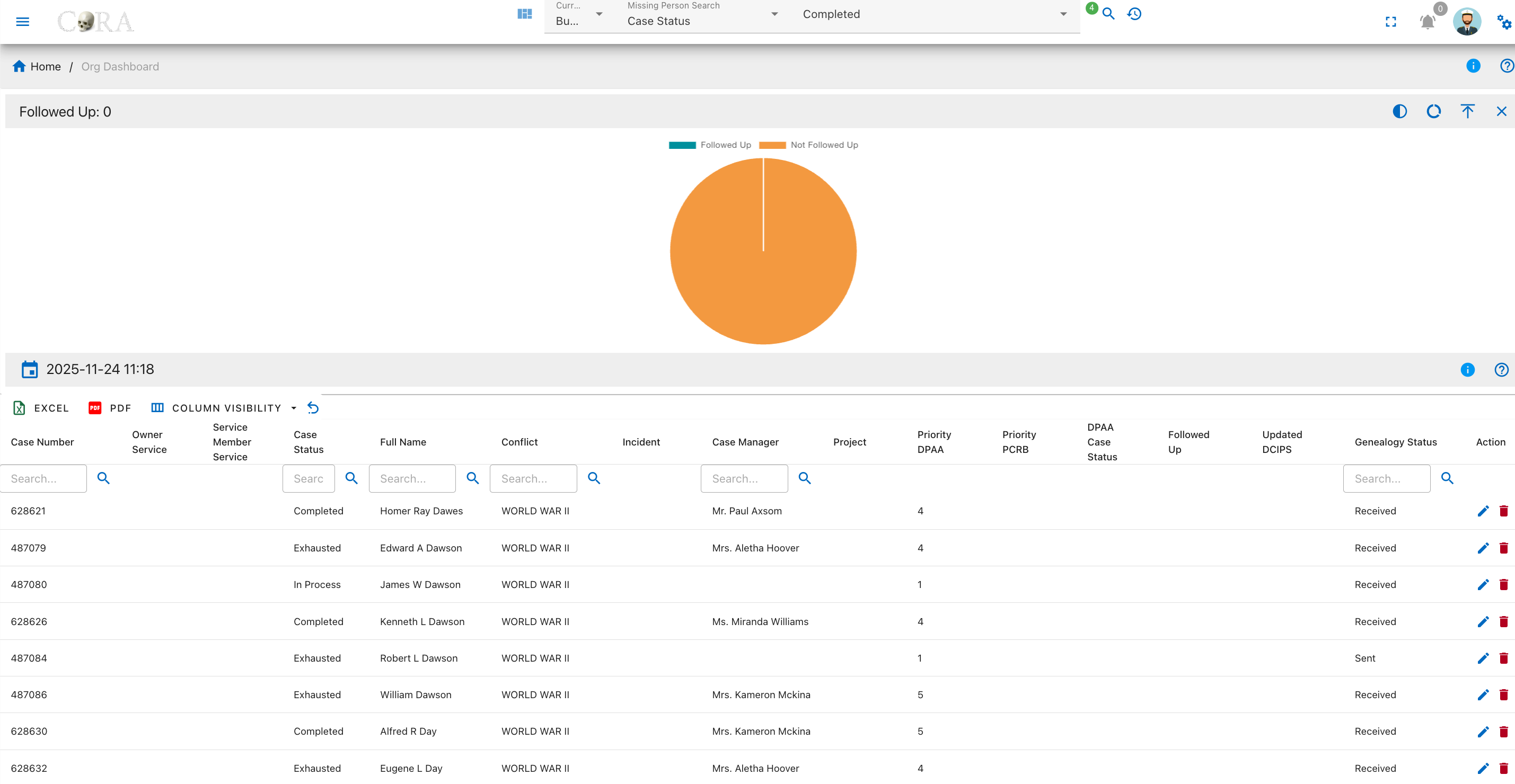
Overview
A pie chart on this page visualizes whether follow-up actions have been completed. The status categories are:
- Followed Up
- Not Followed Up
The legend differentiates completed from pending follow-ups, and tooltips display the number of cases in each.
Updated DCIP
This page provides a summary and tracking interface for the DCIP update status for all missing person cases. The drilldown features an interactive pie chart and a comprehensive data table, allowing users to evaluate which cases have up-to-date DCIP records and which do not.
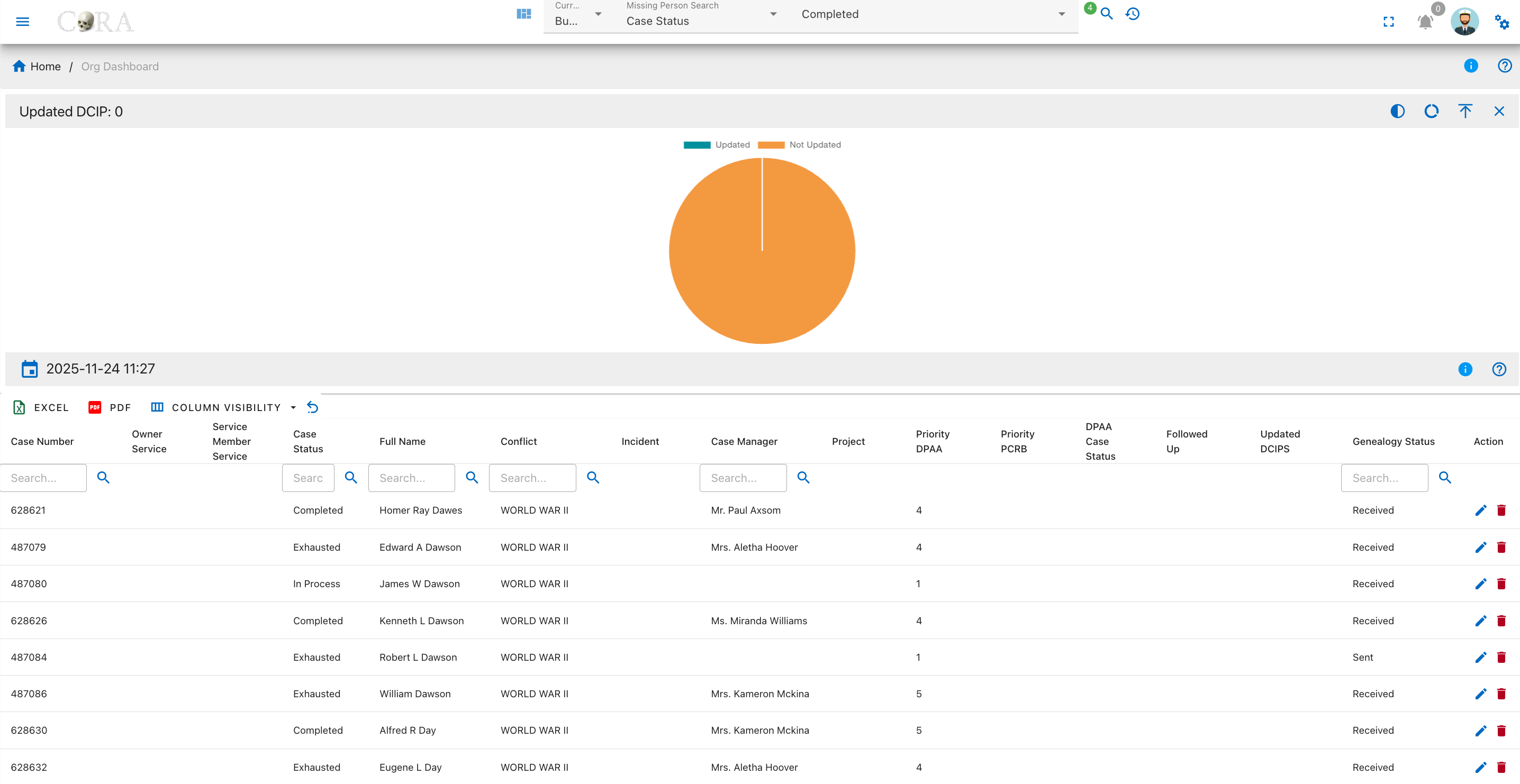
Overview
A pie chart on this page displays the update status for DCIP records. The categories are:
- Updated
- Not Updated
The chart legend identifies each status, and tooltips provide the exact number of cases for each.
IDPF Status
This page provides an overview and detailed tracking for the IDPF request status associated with missing person cases. The drilldown features an interactive pie chart and a searchable, filterable data table to help users monitor which IDPFs have been requested, received, or are not available.
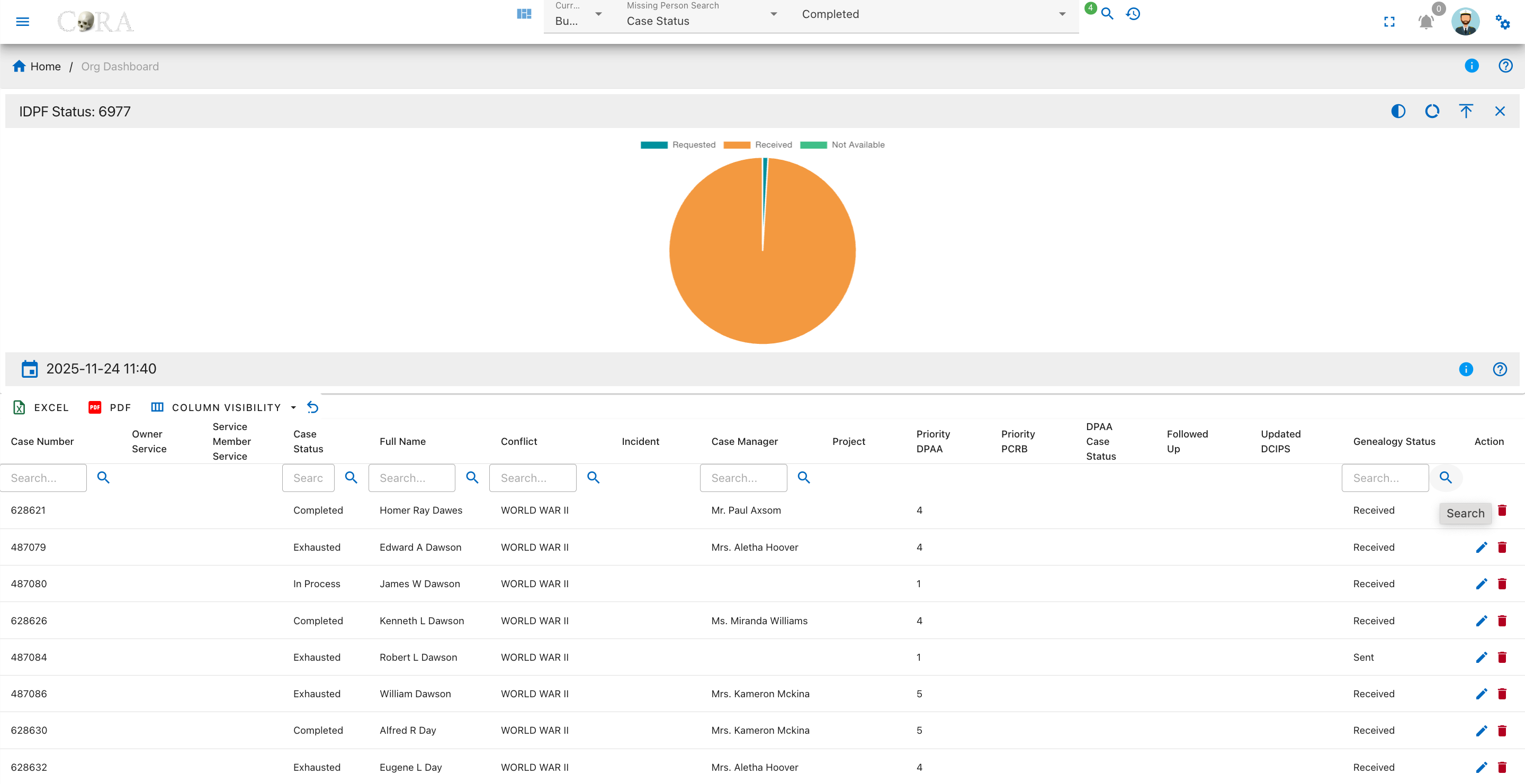
Overview
A pie chart on this page visualizes the request status for Individual Deceased Personnel Files. The categories are:
- Requested
- Received
- Not Available
The legend clarifies each segment, and tooltips show the precise number of cases.
Conflict
This page presents an analysis of the conflict or mission associated with all missing person cases. Users can visualize the distribution of cases by conflict type using an interactive pie chart, and review detailed case information in a searchable, filterable data table.
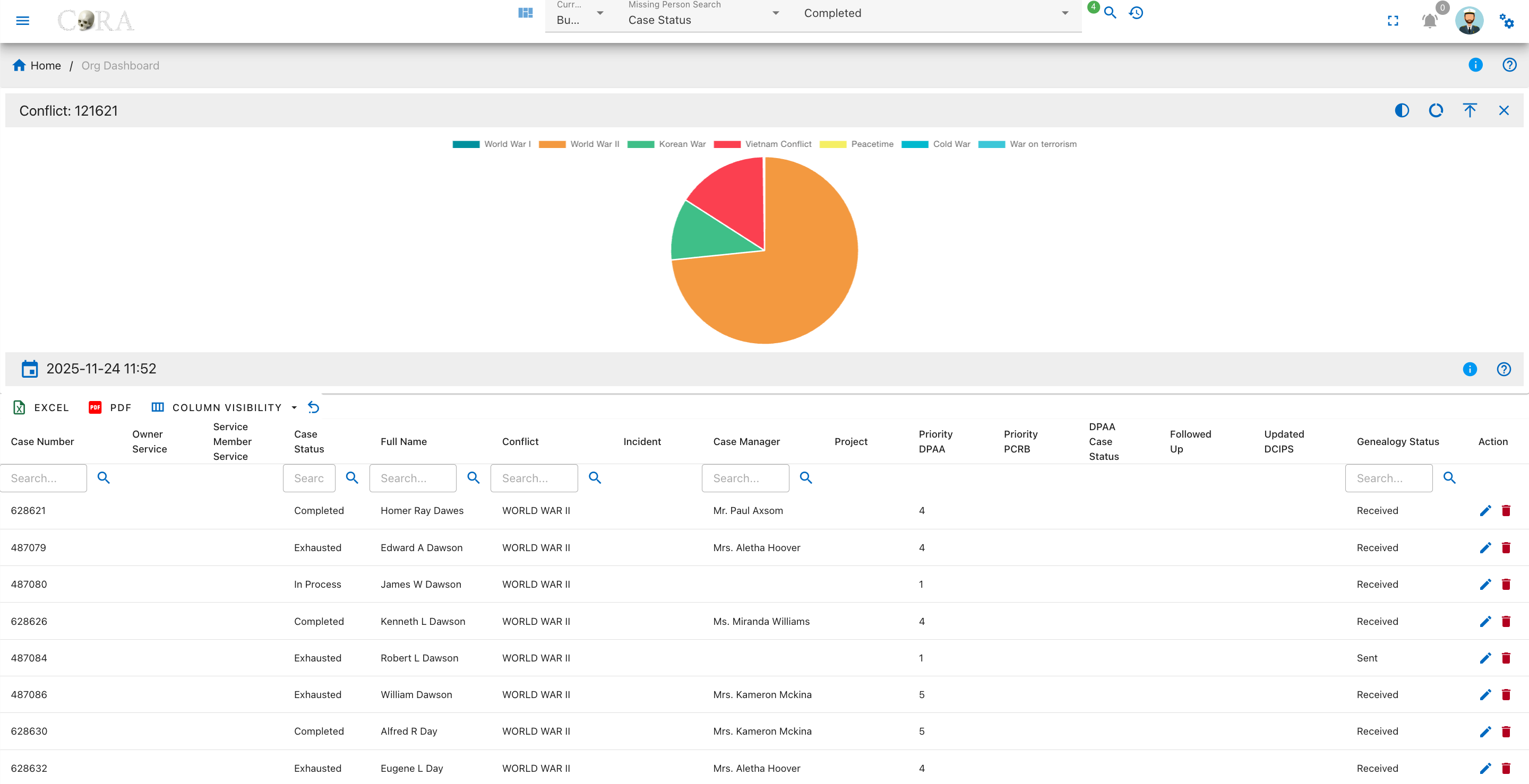
Overview
A pie chart on this page displays how cases are distributed by conflict or mission type. The categories are:
- World War I
- World War II
- Korean War
- Vietnam Conflict
- Peacetime
- Cold War
- War on Terrorism
The legend describes each colored segment, and tooltips reveal the number of cases per conflict.
Case Managers
This page summarizes the distribution of missing person cases assigned to each case manager. The drilldown features an interactive bar chart displaying case volume by manager and a sortable table showing totals for each individual assigned.
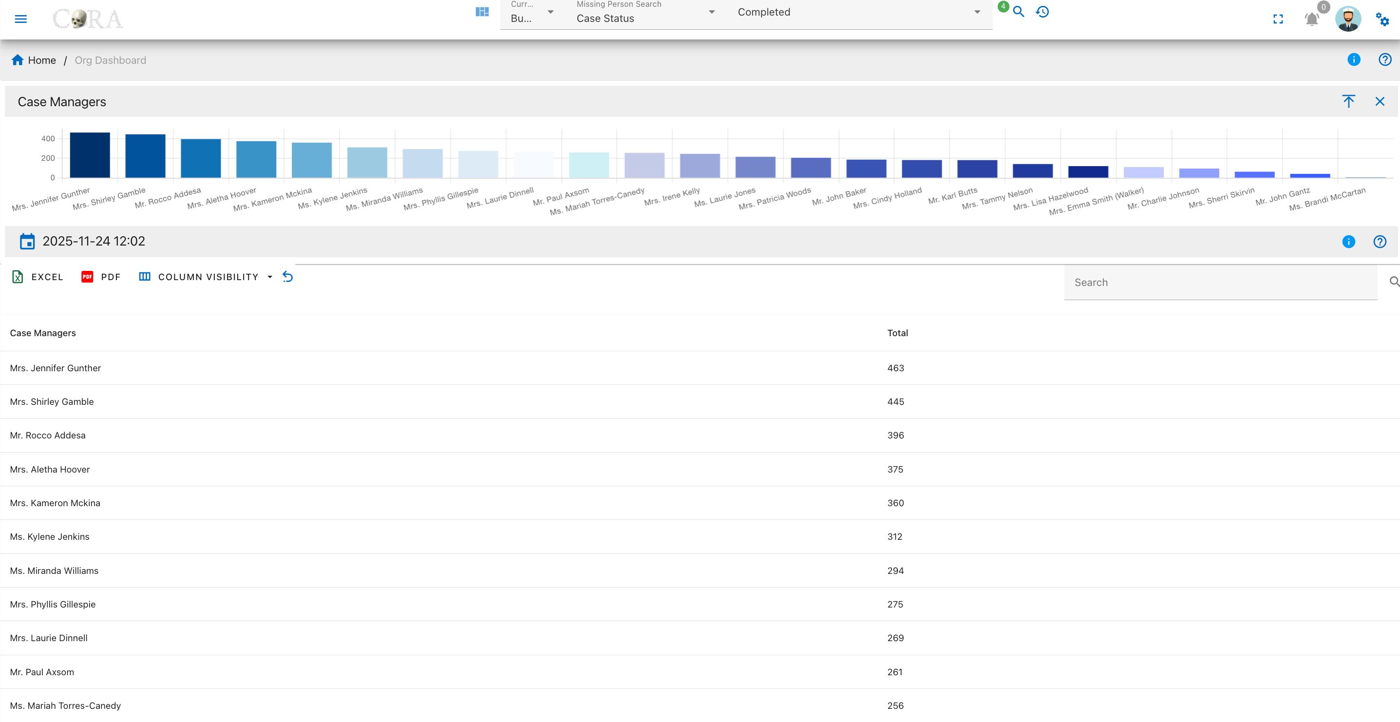
Overview
A bar chart on this page shows the total number of missing person cases assigned to each case manager. The table lists two fields for each manager:
- Case Manager
- Total
The chart legend labels each manager, and tooltips display the precise number of cases assigned to each manager when you hover over a bar.
Table Fields
Below the chart is a searchable, filterable table with key details for each case:
- Case Manager: The staff member assigned to missing person cases.
- Total: The number of cases assigned to that manager.
User Actions
- Searching: Use the search box to find managers by name.
- Sorting: Click any column header to sort the table data.
- Exporting: Download table data to Excel or PDF.
- Column Visibility: Choose which columns are displayed using the column visibility dropdown.
- Refresh: Reload the table using the refresh icon.
Specimen Dashboard Drilldowns
Warning
This page is work in progress.
The dashboard drilldown page provides information on the the drilldown charts and graphs from the dashboard.
File Export Import
File Export, Import and Manager
Data can be exported from and imported into CoRA via the File Export/Import and File Manager system. Options for File Export and Import can be viewed under the left navigation bar. This capability is different from the Excel and PDF export that you will find on all data tables within CoRA such as with Search screens and Reports screens.
File Export
In order to export data from CoRA, navigate to Left Sidebar Menu -> File Export/Import-> File Export. Please note that users can only export data for the current project.
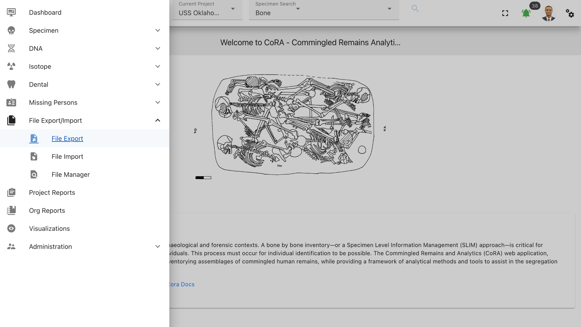
This will take you to the File Export page. This page lists the different types of files exports available in CoRA.
Export Types
The available type of exports and their descriptions are shown in the below table
| Export Type | Description |
|---|---|
| Base - All | Base tables that hold descriptive data for CoRA |
| All | Specimens and all its associations |
| DNA | Specimens, DNA and all DNA associations |
| Measurements | Specimens and all its measurements |
| Zones | Specimens and all its zones |
| Associations | Specimens and its pair, articualtion and refit associations |
| Pairs | Specimens and all its pairs |
| Articulations | Specimens and all its articulations |
| Refits | Specimens and all its refits |
| Taphonomies | Specimens and all its taphonomies |
| Pathology All | Specimens and all its pathology, trauma and anomaly associations |
| Pathology | Specimens and all its pathologies |
| Trauma | Specimens and all its traumas |
| Anomaly | Specimens and all its anomalies |
| Methods | Specimens, its methods and method features |
| Missing Persons | Missing Persons, and Genealogy |
| Instruments | Instruments |
| Osteometric Sorting | Bones and all its measurements |
Export types options available to different role
| Role | Available Export Type |
|---|---|
| anthropologist | Base - All, All, DNA, Measurements, Zones, Associations, Pairs, Articulations, Refits, Taphonomies, Pathology All, Pathology, Trauma, Anomaly, Methods, Instruments, Osteometric Sorting |
| org administrator | Base - All, All, DNA, Measurements, Zones, Associations, Pairs, Articulations, Refits, Taphonomies, Pathology All, Pathology, Trauma, Anomaly, Methods, Missing Persons, Instruments, Osteometric Sorting |
| mp administrator | Missing Persons |
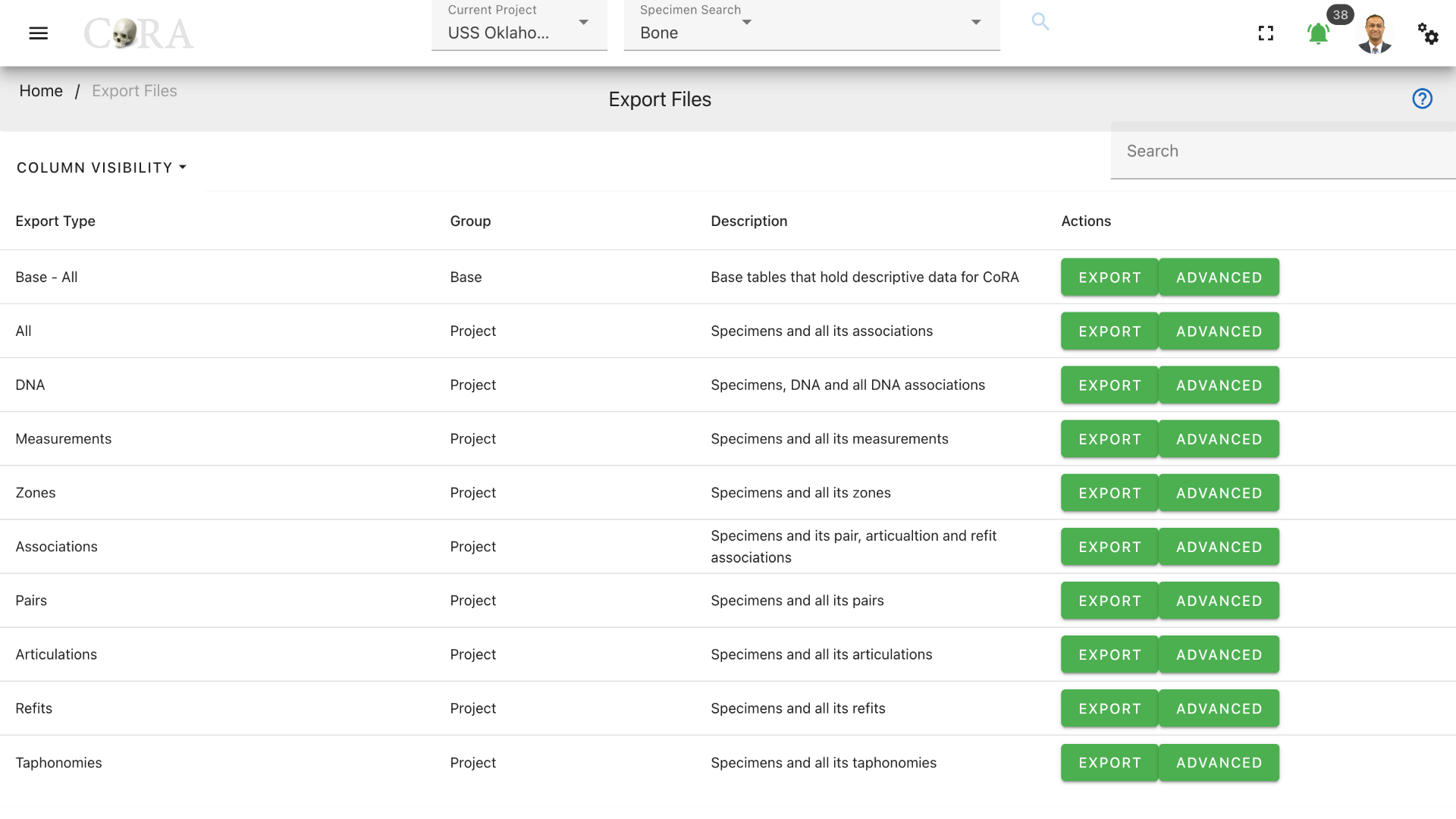
Osteometric Sorting
Osteometric sorting uses size and shape to separate bones from one another. Several statistical methods exist; some references for osteometric sorting are shown below.
References for osteometric sorting
- Byrd, John E., and Bradley J. Adams. "Osteometric sorting of commingled human remains." Journal of forensic sciences 48.4 (2003): 717-724.
- Lynch, Jeffrey James, John Byrd, and Carrie B. LeGarde. "The power of exclusion using automated osteometric sorting: pair‐matching." Journal of forensic sciences 63.2 (2018): 371-380.
- Warnke‐Sommer, Julia D., et al. "Z‐transform method for pairwise osteometric pair‐matching." Journal of forensic sciences 64.1 (2019): 23-33.
CoRA produces a zip file of osteometric sorting bone measurement files for all long bones. Any osteometric sorting program used to process these files must accept the following fields.
| Attribute | Description |
|---|---|
| se_id | The specimen or skeletal element id within CoRA |
| skeletal_element | The composite key the specimen or skeletal element |
| accession_number | The accession number for the specimen |
| provenance1 | The provenance1 for the specimen |
| provenance2 | The provenance2 for the specimen |
| designator | The designator for the specimen |
| skeletal_bone | The skeletal bone type |
| side | The side: right, left, unsided |
| measurements | Example measurement headers for the femur: Fem_01, Fem_02, Fem_03, Fem_04, Fem_05, Fem_06, Fem_07 |
Tip
Use the osteometric sorting export to download bone measurements formatted for input into the osteometric sorting tools.
CoRA creates a background job for the file export process. A notification will appear when the job has completed. You may need to refresh your screen to see the notification. The notification will indicate whether your export was successful or not. The exported records will appear in CoRA under File manager Section.
File Export Notification
Clicking on a file export button will not result in an immediate file(s) download. Instead, a request is made to CoRA to begin a file export job in the background. This may take several minutes depending on the number of records to be exported and the number of background jobs that are currently queued in CoRA. Once the file export job is competed a real-time notification will be seen under the notifications bell located on the top right header of the CoRA application.
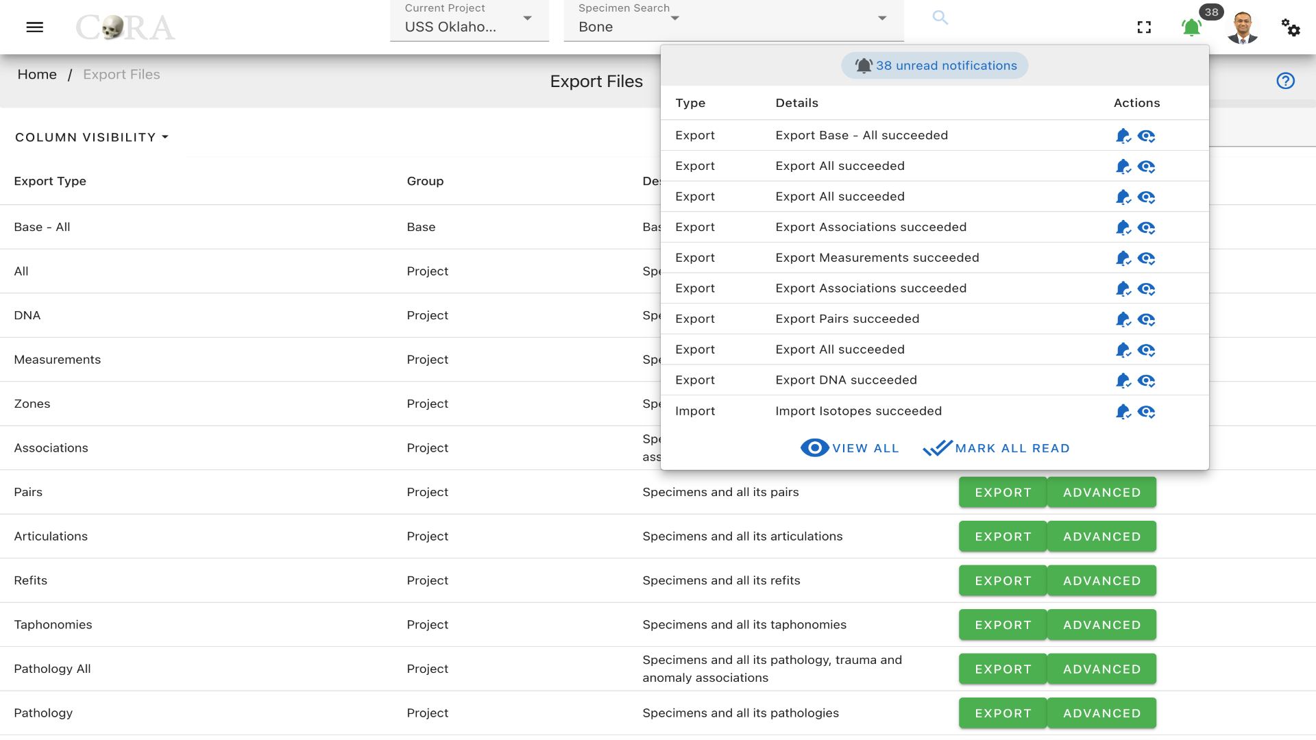
To get rid of the notification, click on mark as read.
Advanced Exports Feature
The anthropologist and mp admin role can only see the export button option, which will export the entire column from that table. The org admin role had both the export and advanced button. The feature of the advanced button is that we can export specific columns from that table to export. Selecting the include timestamp check box, adds the four columns 'created_by, created_at, updated_by, updated_at, deleted_at' in the excel.

Click on 'Export Tables' to start the export for those particular tables and columns.
File Manager
All files exported and imported into CoRA can be accessed at a central location called the File Manager. The file(s) that you just exported will be located here after CoRA completes the file export job. To access the File Manager, navigate to Left Sidebar Menu -> File Export/Import-> File Manager.
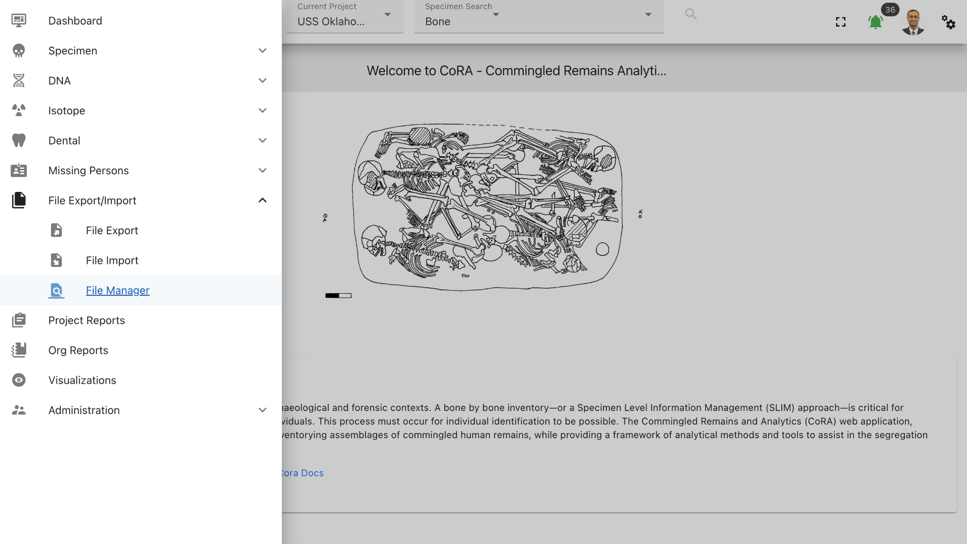
The File Manager will list all the file export/import jobs that have been completed by CoRA with most recent export/import jobs listed first. To download a file export, click download. A file export does not become available on this page until the requested file export job has been completed by CoRA.
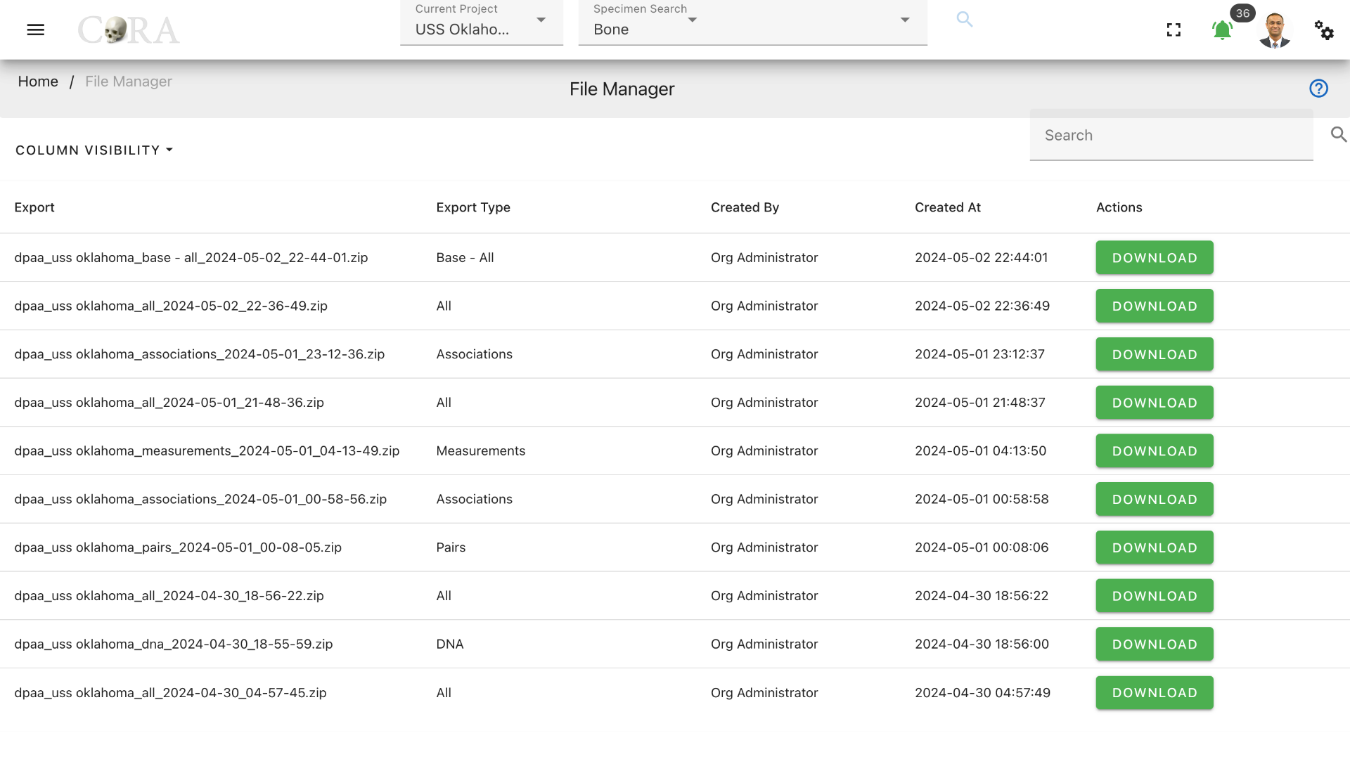
Click on the 'Download' button in green to download the particular files exported to CoRA.
File Import
In order to import a file, navigate to Left Sidebar Menu -> File Export/Import-> File Import
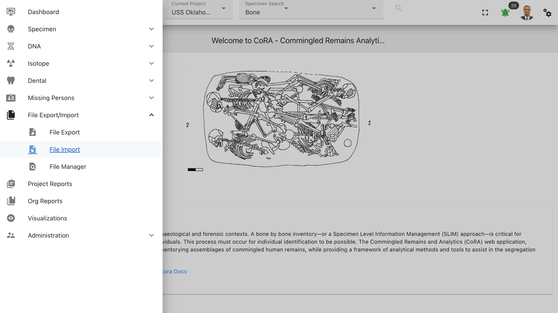
On the file import screen, select the import file type that you wish to upload. A template can be downloaded for the file type that you are importing. CoRA will not allow you to import a file unless the file import type is selected.
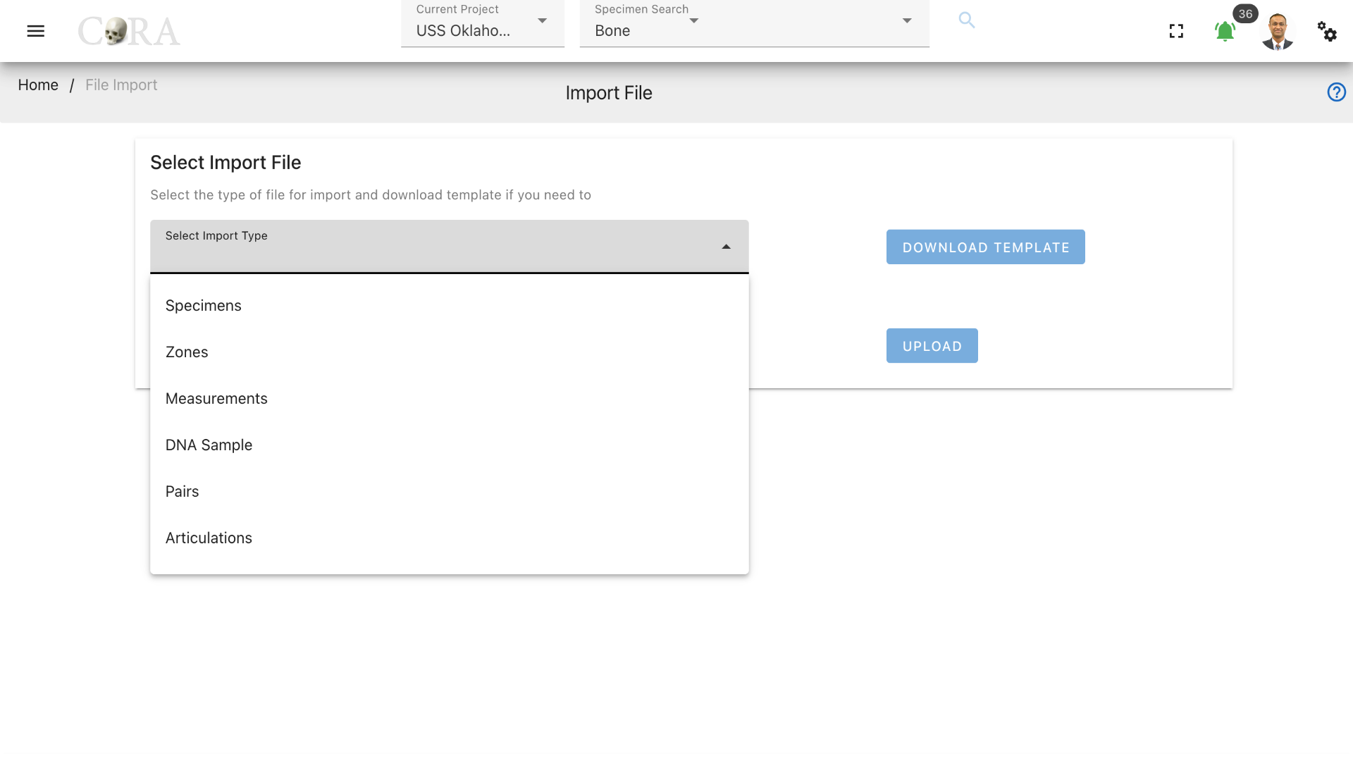
The pairs file type is shown as selected in the screenshot below. Click on browse to select a file to upload from your computer. Once selected, hit upload to upload the file to CoRA.
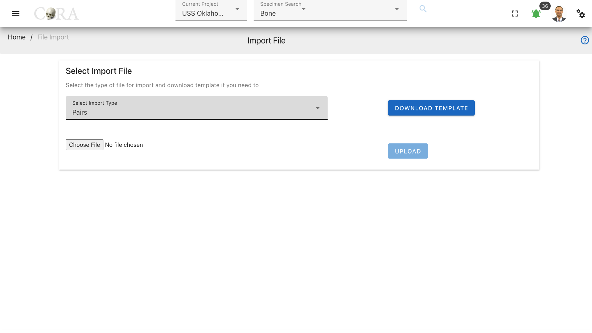
As with file export, CoRA creates a background job for the file import process. A notification will appear when the job has completed. You may need to refresh your screen to see the notification. The notification will indicate whether your import was successful or not. The imported records will appear in CoRA after a successful import. Click on 'view notification' to read the import information in detail.
Import Types
This section details the type of file import types available to the user. Templates can be downloaded for each import file type on the file import page. Following are the import types that are available to the user.
- Specimens
- Zones
- Measurements
- DNA sample
- Pairs (Results From Osteometric Sorting Tools)
- Articulations (Results From Osteometric Sorting Tools)
- DNA
- Isotopes
- Missing Persons
- Missing Persons-DCIPS
- External Systems - Specimens & DNA sample
- External Systems - Specimens
- External Systems - DNA sample
The file being imported must contain a specific word depending on the import type. The filename can contain other words and characters, but it must contain one of the following words.
| Import Type | Required Word |
|---|---|
| Specimens | specimens |
| Zones | zone |
| Measurements | measurement |
| DNA | dna |
| DNA Sample | dna |
| Pairs | pair |
| Articulations | articulation |
| Missing Persons | missing / dcips |
| Missing Persons - DCIPS | dcips |
| Isotopes | Isotope |
| External Systems - Specimen and DNA | externalsystem |
| External Systems - Specimen | externalse |
| External Systems - DNA | externaldna |
Import types options available to different role
| Role | Available Import Type |
|---|---|
| anthropologist | Specimens,Zones,Measurements,DNA, DNA Sample, Isotopes, Pairs, Articulations, External Systems - Specimens & DNA, External Systems - Specimens, External Systems - DNA |
| org administrator | Specimens,Zones,Measurements,DNA,Pairs,Articulations,Missing Persons, Missing Persons-DCIPS, External Systems - Specimens & DNA, External Systems - Specimens, External Systems - DNA |
| mp administrator | Missing Persons, Missing Persons-DCIPS |
File Upload
Click on browse to select a file to upload from your computer. Once selected, click upload to upload the file to CoRA. The upload button will be disabled until the import type selected and file is attached. Both are the mandatory input for the upload to get triggered.
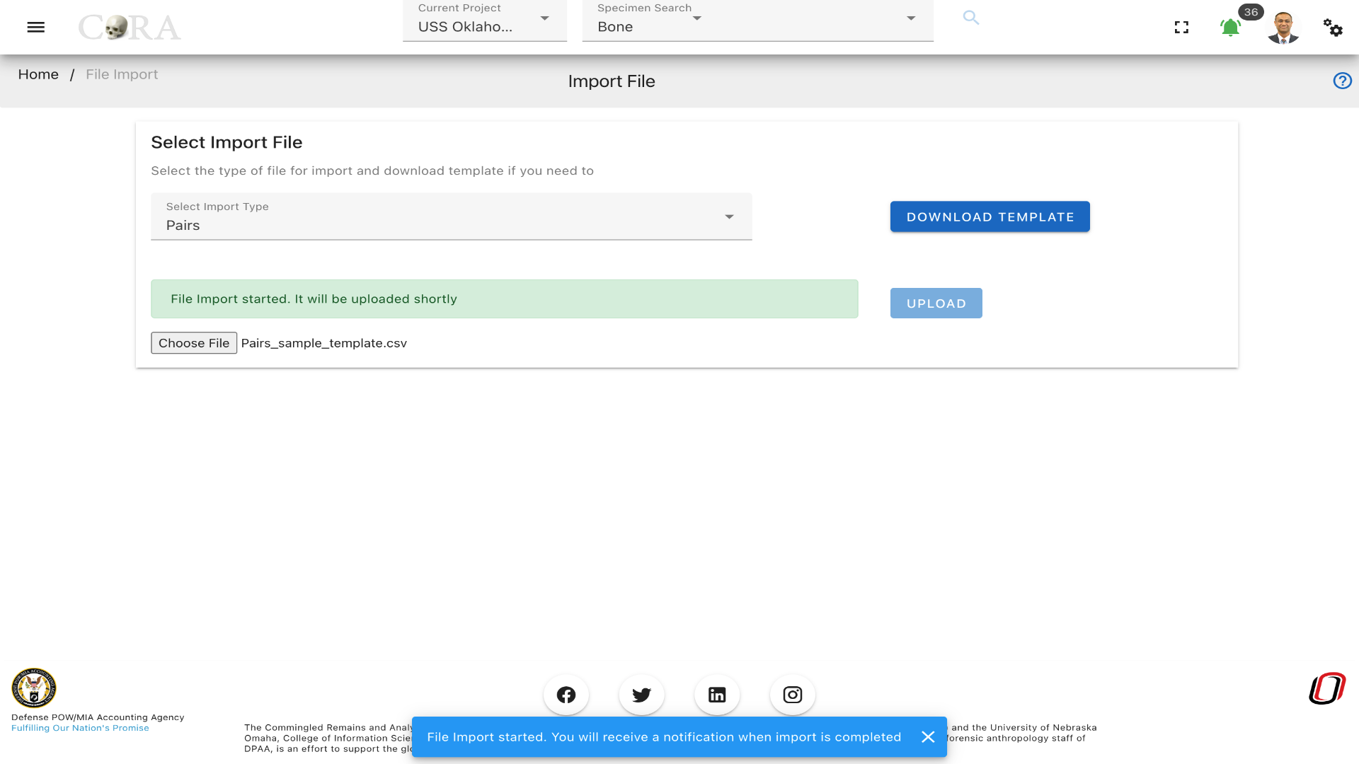
Tip
CoRA validates that the type chosen and file name attached match, it will throws an error if they don't match.
File Upload - External Systems
Data can also be imported from external systems for DNA and Skeletal elements. The column names mapping from external systems to CoRA is shown below.
DNA
Data in a row is mapped to DNA if the value of the 'progname' column in the external systems is 'DNA Sample'.
| External Systems | DNA (CoRA) |
|---|---|
| org_id | org_id |
| project_id | project_id |
| afdil_case_no | external_case_id |
| afdil_sample_no | sample_number |
| priority | priority |
| mito_sequence_number | mito_sequence_number |
| mito_sequence_subgroup | mito_sequence_subgroup |
| mito_sequence_similar | mito_sequence_similar |
| mito_match_count | mito_match_count |
| mito_total_count | mito_total_count |
| mito_receive_date | mito_receive_date |
| mito_haplogroup_id | mito_haplogroup_id |
| analysis_type_id | analysis_type_id |
| mito_results_confidence | mito_results_confidence |
| mito_num_loci | mito_num_loci |
| progname (checks conditions) | sbId |
| austr_match_count | austr_match_count |
| austr_total_count | austr_total_count |
| austr_num_loci | austr_num_loci |
| ystr_match_count | ystr_match_count |
| ystr_total_count | ystr_total_count |
| ystr_num_loci | ystr_num_loci |
| ystr_haplogroup | ystr_haplogroup |
| mito_mcc_date | mito_mcc_date |
| priority_date | priority_date |
| btb_request_date | btb_request_date |
| btb_results_date | btb_results_date |
| mito_request_date | mito_request_date |
| austr_request_date | austr_request_date |
| austr_receive_date | austr_receive_date |
| austr_mcc_date | austr_mcc_date |
| ystr_request_date | ystr_request_date |
| ystr_receive_date | ystr_receive_date |
| ystr_mcc_date | ystr_mcc_date |
| mito_fasta_sequence | mito_fasta_sequence |
| uuid | uuid |
| mito_confirmed_regions | mito_confirmed_regions |
| mito_base_pairs | mito_base_pairs |
| locus | locus |
| weight_sample_remaining | weight_sample_remaining |
| notes | notes |
| mito_method | mito_method |
| external_sample_number | external_sample_number |
| dispostion_of_evidence | dispostion_of_evidence |
| disposition | disposition |
| sample_condition | sample_condition |
| mito_polymorphisms | mito_polymorphisms |
| austr_method | austr_method |
| austr_results_confidence | austr_results_confidence |
| austr_sequence_number | austr_sequence_number |
| austr_sequence_subgroup | austr_sequence_subgroup |
| austr_sequence_similar | austr_sequence_similar |
| austr_loci | austr_loci |
| ystr_method | ystr_method |
| ystr_results_confidence | ystr_results_confidence |
| ystr_sequence_number | ystr_sequence_number |
| ystr_sequence_subgroup | ystr_sequence_subgroup |
| ystr_sequence_similar | ystr_sequence_similar |
| ystr_loci | ystr_loci |
| custom_field_1 | custom_field_1 |
| custom_field_2 | custom_field_2 |
| custom_field_3 | custom_field_3 |
| mito_haplosubgroup | mito_haplosubgroup |
| ystr_haplosubgroup | ystr_haplosubgroup |
| additional_testing | additional_testing |
| resample_indicator | resample_indicator |
| exhibitcreatedby | created_by |
| exhibitcreatedby | updated_by |
Skeletal Elements
Data is mapped to skeletal elements if 'progname' column of external systems is not 'DNA Sample'.
| External Systems | DNA (CoRA) |
|---|---|
| casenumber | accession_number |
| crimesceneid | provenance 1 |
| location_found | provenance 2 |
| exhibitno | designator |
| user_id | user_id |
| org_id | org_id |
| project_id | project_id |
| side | side |
| progname (checks conditions) | sb_id |
| inv_completeness | completeness |
| measured | measured |
| dna_sampled | dna_sampled |
| ct_scanned | ct_scanned |
| xray_scanned | xray_scanned |
| clavicle_triage | clavicle_triage |
| inventoried | inventoried |
| reviewed | reviewed |
| casenumber & exhibitno | external_id |
| individual_number | individual_number |
| inventoried_at | inventoried_at |
| reviewed_at | reviewed_at |
| consolidated_on | consolidated_on |
| isotope_sampled | isotope_sampled |
| count | count |
| mass | mass |
| bone_group_id | bone_group_id |
| inventoried_by_id | inventoried_by_id |
| remains_status | remains_status |
| remains_release_date | remains_release_date |
| identification_date | identification_date |
| 3D_scanned | 3D_scanned |
| notes | notes |
| uuid | uuid |
| ct_scanned_date | ct_scanned_date |
| xray_scanned_date | xray_scanned_date |
| 3D_scanned_date | 3D_scanned_date |
| min_age | min_age |
| max_age | max_age |
| custom_field_1 | custom_field_1 |
| custom_field_2 | custom_field_2 |
| custom_field_3 | custom_field_3 |
| exhibitcreatedby | created_by |
| exhibitcreatedby | updated_by |
File Import Notification
As with file export, CoRA creates a background job for the file import process. A notification will appear when the job has completed. You may need to refresh your screen to see the notification. The notification will indicate whether your import was successful or not. The imported records will appear in CoRA after a successful import. You can click the eye icon under the Action menu to see the detailed result of the import process. It explains how many records were successfully imported and if there were failures it will also provide the reason for the failure rows. Click the green bell sign in the top right corner to view and mark all notifications.
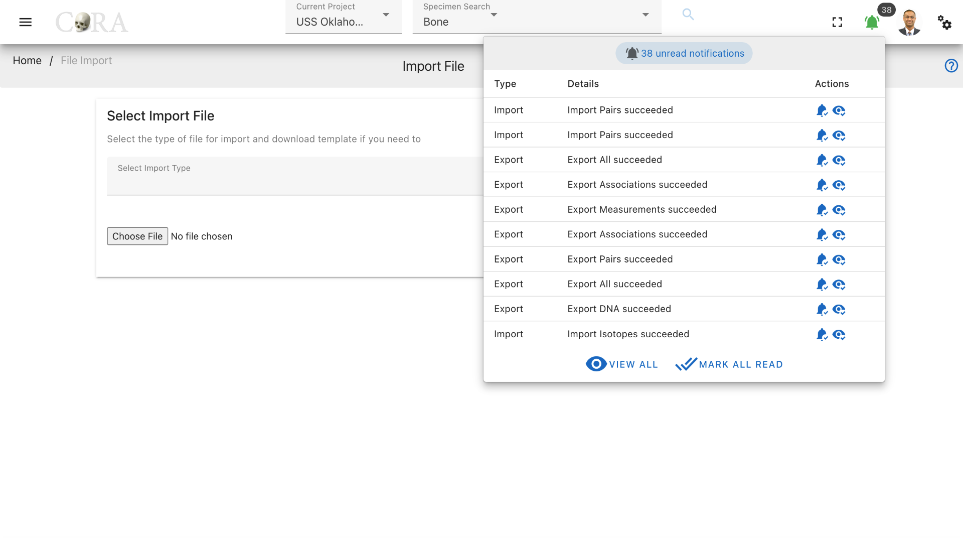
Osteometric Sorting
Pairs
A pairs file produced by an osteometric sorting program must have the following fields for upload to CoRA. Only pairs that were not excluded should be uploaded to CoRA.
| Attribute | Description |
|---|---|
| se_id | The specimen or skeletal element id internal to CoRA. |
| pair_id | The specimen or skeletal element id internal to CoRA for the paired element |
| se_skeletal_element | The composite key for the specimen |
| se_accession_number | The accession number for the specimen |
| se_provenance1 | The provenance1 for the specimen |
| se_provenance2 | The provenance2 for the specimen |
| se_designator | The designator for the specimen |
| pair_skeletal_element | The composite key for the paired specimen |
| pair_accession_number | The accession number for the paired specimen |
| pair_provenance1 | The provenance1 for the paired specimen |
| pair_provenance2 | The provenance2 for the paired specimen |
| pair_designator | The designator for the paired specimen |
| bonename | The specimen bone type |
| compare_method | The osteometric sorting method used |
| compare_method_settings | Program settings |
| sample_size | The size of the reference sample |
| pvalue | The p-value of the statistical test |
| num_measurements | Number of measurements used for the comparison |
| measurements_used | The measurements that were used |
| measurement_means | The means of the measurements in the reference population |
| measurement_sd | The standard deviation of the measurements |
Articulations
A articulations file produced by an osteometric sorting program must have the following fields for upload to CoRA. Only articulations that were not excluded should be uploaded to CoRA.
| Attribute | Description |
|---|---|
| se_id | The specimen or skeletal element id internal to CoRA. |
| articulation_id | The specimen or skeletal element id internal to CoRA for the articulated element |
| se_skeletal_element | The composite key for the specimen |
| se_accession_number | The accession number for the specimen |
| se_provenance1 | The provenance1 for the specimen |
| se_provenance2 | The provenance2 for the specimen |
| se_designator | The designator for the specimen |
| articulation_skeletal_element | The composite key for the articulated specimen |
| articulation_accession_number | The accession number for the articulated specimen |
| articulation_provenance1 | The provenance1 for the articulated specimen |
| articulation_provenance2 | The provenance2 for the articulated specimen |
| articulation_designator | The designator for the articulated specimen |
| bonename | The specimen bone type |
| compare_method | The osteometric sorting method used |
| compare_method_settings | Program settings |
| sample_size | The size of the reference sample |
| pvalue | The p-value of the statistical test |
| num_measurements | Number of measurements used for the comparison |
| measurements_used | The measurements that were used |
| measurement_means | The means of the measurements in the reference population |
| measurement_sd | The standard deviation of the measurements |
Missing Persons DCIPS Import
There is currently an issue affecting the Missing Persons DCIPS import. No more than 20,000 rows can be imported at one time, and the fields in the excel file generated by DCIPS are inaccurate.
Less than 20,000 rows at a time must be taken from the DCIPS excel file and pasted into the Missing Persons template. The import must then be run until all the fields have been imported. Currently, there are about 130,000 rows exported from DCIPS, and the import process requires seven separate files.
Another possible solution is to obtain a delta file containing only the changes from the last import. This approach has not yet been tested.
Mobile Readiness
Mobile Readiness
CoRA has been designed as a web responsive application which is mobile ready from the get go. This means you can serve your project needs with confidence – the underlying layout, screens, widgets, styles and user interface automatically adapts to perfectly fit the available screen real estate, no matter the type or size of the viewing device. CoRA allows users to access the application and use the full range of features with responsiveness, flexibility, and extensibility.
– CoRA works where you are, on any device
What devices does CoRA support?
CoRA Works on all devices
Device Sizes
| Device | Size | Screen size |
|---|---|---|
| Mobile | Small | 320px |
| Mobile | Medium | 375px |
| Mobile | Large | 425px |
| Tablet | 786px | |
| Laptop | Small | 1024px |
| Laptop | Large | 1440px |
Tip
For smartphones & tablet sizes and under, the top right side navbar will be displayed as a condensed hamburger menu
Login
- Mobile - 320px, 375px and 425px
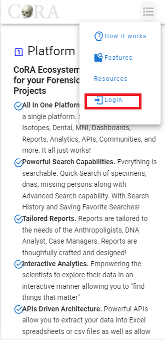
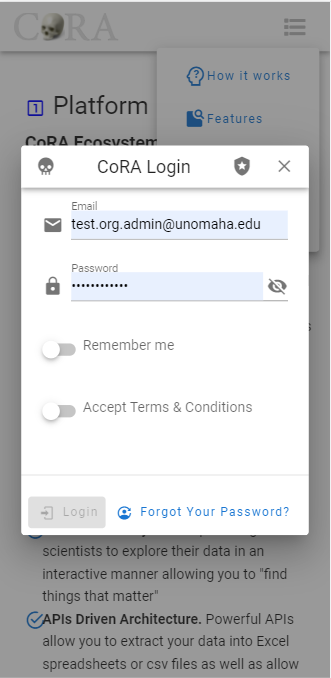
- Tablet - 768px
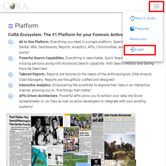
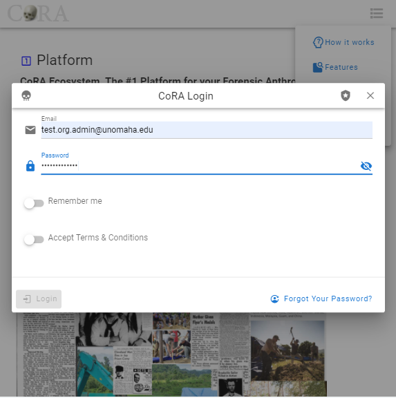
- Laptop - 1024px
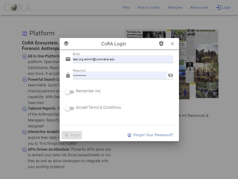
- Large Laptop - 1440px
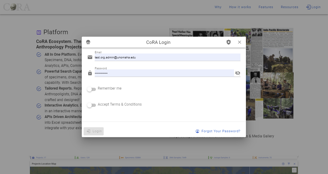
Dashboard
- Mobile - 320px, 375px and 425px
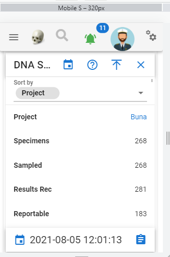
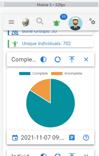
- Tablet - 768px
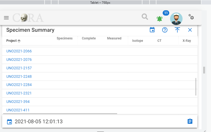
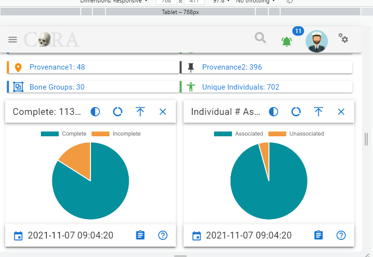
- Laptop - 1024px
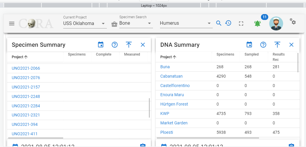
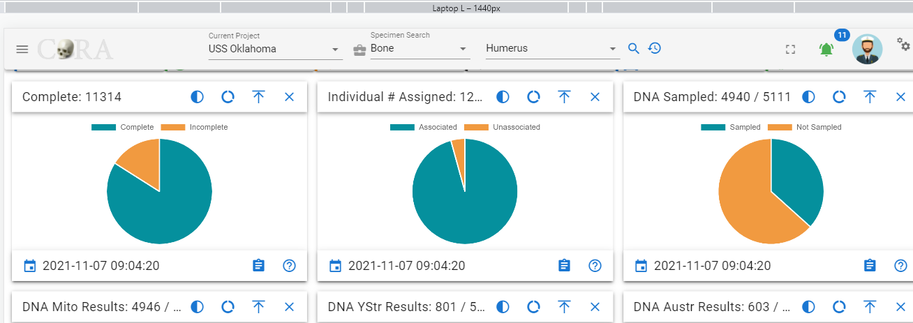
Search
- Mobile - 320px, 375px and 425px
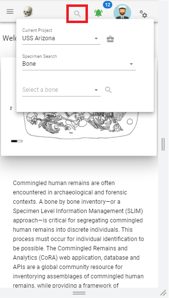
- Tablet - 768px
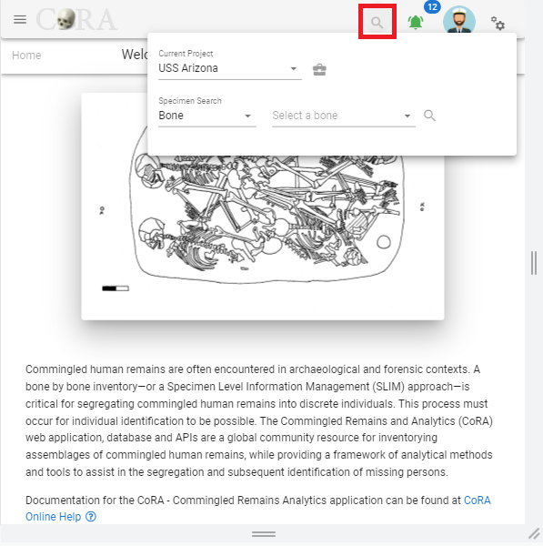
- Laptop - 1024px
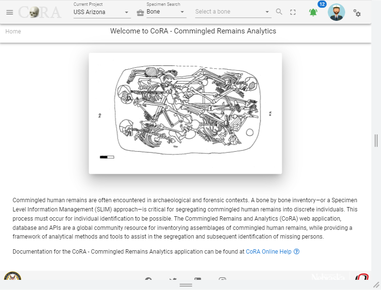
- Large Laptop - 1440px
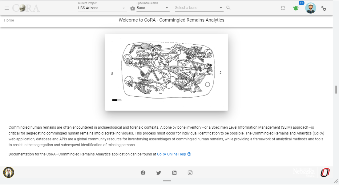
Specimens
- Mobile - 320px, 375px and 425px
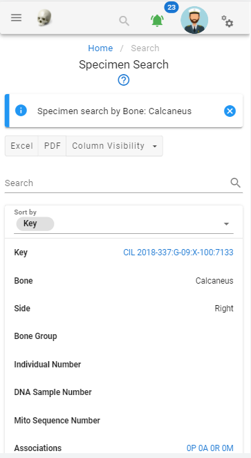
- Tablet - 768px
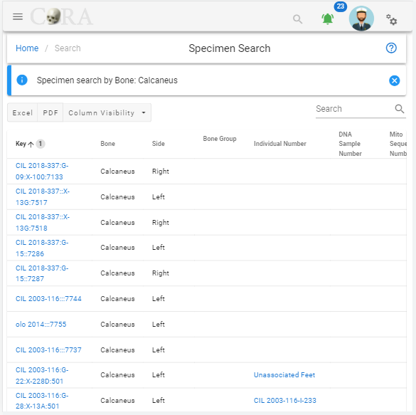
- Laptop - 1024px
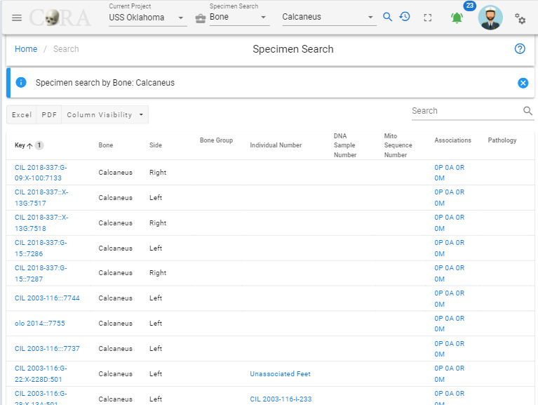
- Large Laptop - 1440px
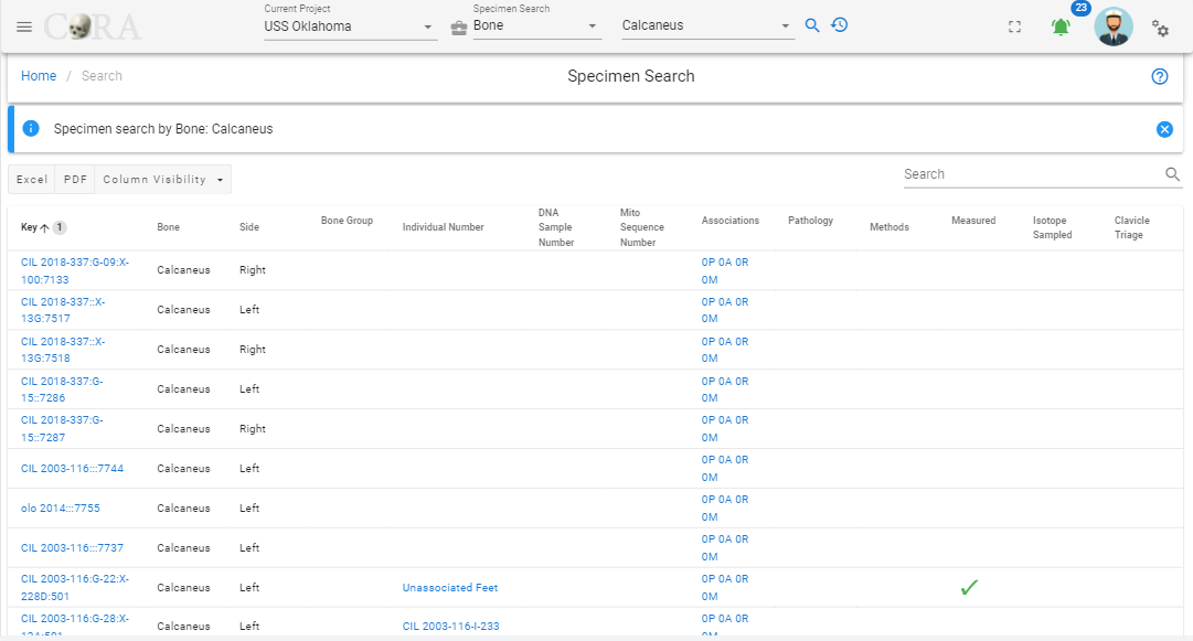
Forensic Anthro Guide
Anomaly
In this section we present the anomalies available within CoRA for assignment to individual specimens. Anomalies are organized by Bone
How can I add new anomalies to CoRA?
You can request new anomalies to be added to CoRA if the one you are looking for is not present by creating an issue on our issue tracker.
Calcaneus
| Individuating Trait |
|---|
| Anterior facet double |
| Shape of talar articular surface |
Cervical vertebra 1
| Individuating Trait |
|---|
| Bifurcate foramen transversarium |
| Incomplete foramen transversarium |
| Retroarticular bridge |
Cervical vertebra 2
| Individuating Trait |
|---|
| Bifurcate foramen transversarium |
| Open foramen transversarium |
Cervical vertebra 3
| Individuating Trait |
|---|
| Accessory transverse foramen |
Cervical vertebra 4
| Individuating Trait |
|---|
| Accessory transverse foramen |
Cervical vertebra 5
| Individuating Trait |
|---|
| Accessory transverse foramen |
Cervical vertebra 6
| Individuating Trait |
|---|
| Accessory transverse foramen |
Cervical vertebra 7
| Individuating Trait |
|---|
| Accessory transverse foramen |
| Vertebral shift |
Clavicle
| Individuating Trait |
|---|
| Rhomboid fossa |
Cranium
| Individuating Trait |
|---|
| Accessory infra-orbital foramen |
| Accessory lesser palatine foramen |
| Anterior ethmoid foramen |
| Asterion ossicle |
| Auditory torus |
| Bregmatic bone |
| Condylar facet |
| Coronal ossicle |
| Deviated nasal septum |
| Epipteric bone |
| Foramen ovale incomplete |
| Foramen of Huschke |
| Foramen spinosum open |
| Frontal foramen |
| Fronto-temporal articulation |
| Lambda ossicle |
| Lambdoidal suture ossicle |
| Mastoid foramen exsutural |
| Maxillary torus |
| Metopism |
| Palatine torus |
| Parietal foramen |
| Parietal notch |
| Posterior condylar canal |
| Posterior ethmoid foramen |
| Precondylar tubercle |
| Supra-orbital foramen |
| Zygomatico-facial foramen |
Ethmoid
| Individuating Trait |
|---|
| Posterior ethmoid foramen |
Femur
| Individuating Trait |
|---|
| Allens fossa |
| Poiriers facet |
| Third trochanter |
Frontal
| Individuating Trait |
|---|
| Anterior ethmoid foramen |
| Frontal foramen |
| Metopism |
| Supra-orbital foramen |
Humerus
| Individuating Trait |
|---|
| Septal aperture |
| Supracondylar process |
Lumbar vertebra 1
| Individuating Trait |
|---|
| Vertebral shift |
Lumbar vertebra 5
| Individuating Trait |
|---|
| Vertebral shift |
Maxilla
| Individuating Trait |
|---|
| Accessory infra-orbital foramen |
| Maxillary torus |
Nasal
| Individuating Trait |
|---|
| Deviated nasal septum |
Occipital
| Individuating Trait |
|---|
| Condylar facet |
| Posterior condylar canal |
| Precondylar tubercle |
Os coxa
| Individuating Trait |
|---|
| Accessory sacroiliac articulation |
| Acetabulum crease |
Palatine
| Individuating Trait |
|---|
| Accessory lesser palatine foramen |
| Palatine torus |
Parietal
| Individuating Trait |
|---|
| Parietal foramen |
Sacrum
| Individuating Trait |
|---|
| Accessory sacroiliac articulation |
| Vertebral shift |
Scapula
| Individuating Trait |
|---|
| Accessory acromion articular facet |
| Circumflex sulcus |
| Glenoid fossa extension |
| Scapular foramen |
| Unfused acromion process |
Sphenoid
| Individuating Trait |
|---|
| Foramen of Huschke |
| Foramen ovale incomplete |
| Foramen spinosum open |
Sternum
| Individuating Trait |
|---|
| Sternal aperture |
Sternal body
| Individuating Trait |
|---|
| Sternal aperture |
Talus
| Individuating Trait |
|---|
| Squatting facets |
Temporal
| Individuating Trait |
|---|
| Auditory torus |
| Mastoid foramen exsutural |
Thoracic vertebra 1
| Individuating Trait |
|---|
| Vertebral shift |
Thoracic vertebra 11
| Individuating Trait |
|---|
| Vertebral shift |
Thoracic vertebra 12
| Individuating Trait |
|---|
| Vertebral shift |
Tibia
| Individuating Trait |
|---|
| Squatting facets |
Ulna
| Individuating Trait |
|---|
| Divided trochlear notch |
Unseriated cervical vertebra
| Individuating Trait |
|---|
| Accessory transverse foramen |
| Bifurcate foramen transversarium |
| Incomplete foramen transversarium |
| Open foramen transversarium |
| Retroarticular bridge |
Zygomatic
| Individuating Trait |
|---|
| Zygomatico-facial foramen |
Measurements
In this section we present the images for measurements used in the inventory of human remains, along with captions and desciptions of each measurement.
Measurement definitions are derived from
- Berg (2014) Biological affinity and sex from the mandible utilizing multiple world populations. In: Berg GE, Ta’ala SC, editors. Biological Affinity in Forensic Identification of Human Skeletal Remains: Beyond Black and White. pp. 43–81.
- Byrd & Adams (2003) Osteometric sorting of commingled human remains. Journal of Forensic Sciences, 48:717-724.
- Langley et al. (2016) Data Collection Procedures for Forensic Skeletal Material 2.0. University of Tennessee and Lincoln Memorial University
- Meadows and Langley (1992) Estimation of stature from metacarpal lengths. Journal of Forensic Sciences, 37:147-154.
Recognition, Kudos and Thanks 🎀
Images by Elizabeth Lockett and Nandar Yukyi are derived from Langley et al. (2016)1.
Cranium
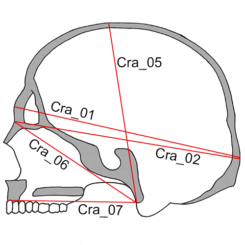
Cra_01 Maximum Cranial Length (g-op, GOL): The straight-line distance from glabella (g) to opisthocranion (op) in the midsagittal plane.
- Instrument: spreading caliper
- Comment: Set the skull on its base. Place one caliper point in the glabellar region in the midline and hold with fingers while the other caliper point is applied to the posterior portion of the skull in the midsagittal plane and moved up and down until the maximum length is obtained. On finding this, move the left point up and down slightly to make sure the reading is maximum (Howells 1973: 170; Martin and Knussmann 1988:168, #1; Moore-Jansen et al. 1994, #1; Langley et al. 2016:65, #1).
Cra_02 Nasio-occipital Length (NOL): Maximum length in the midsagittal plane, measured from nasion (n).
- Instrument: spreading caliper
- Comment: With the skull in position as for Maximum Cranial Length, place the one caliper point at (n) and move the other point along the occiput in the midline for the maximum reading (Howells 1973:171; Langley et al. 2016:65, #2).
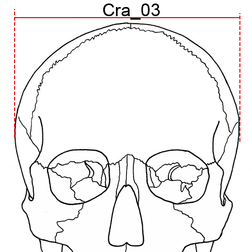
Cra_03 Maximum Cranial Breadth (eu-eu, XCB): The maximum width of the skull perpendicular to the mid-sagittal plane wherever it is located with the exception of the inferior temporal line and the immediate area surround the latter (i.e. the posterior roots of the zygomatic arches and supramastoid crest).
- Instrument: spreading caliper
- Comment: Cra_03 is measured with the skull resting either on its base or on the occiput. The two measuring points (eurya) should lie in the same horizontal and frontal planes. Place the arms of the caliper at the same level while maintaining the hinge joint of the caliper in the mid-sagittal plane. Hold the ends of the caliper in each hand and apply to the lateral portions of the skull, making circular motions. Make sure you include areas below the squamosal suture, where the maximum is sometimes found. (Howells 1973:172; Hrdlicka 1920:14; Martin and Knussmann 1988:170, #8; Moore-Jansen et al. 1994, #2; Langley et al. 2016:65, #3).
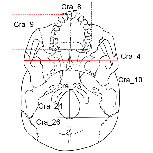
Cra_04 Bizygomatic Breadth (zy-zy, ZYB): The maximum breadth across the zygomatic arches, wherever found, perpendicular to the mid-sagittal plane.
- Instrument: sliding or spreading calipers
- Comment: Place the skull on its occiput, base toward observer, and apply the blunt points of the caliper to the zygomatic arches and locate the maximum breadth perpendicular to the mid-sagittal plane. (Howells 1973:173; Moore-Jansen et al. 1994, #3; Langley et al. 2016:66, #4).
Cra_05 Basion-Bregma Height (ba-b, BBH): The distance from basion (ba) to bregma (b).
- Instrument: spreading caliper
- Comment: Place the skull on its occiput with the right side facing the observer. Apply the endpoint of one of the arms of the caliper at (ba) and support with fingers. Then apply the endpoint of the second arm of the caliper to (b) (Howells 1973:172; Moore-Jansen et al. 1994, #4; Langley et al. 2016:66, #5).
Cra_06 Cranial Base Length (ba-n, BNL): The distance from nasion (n) to basion (ba).
- Instrument: spreading caliper
- Comment: Rest the skull on the cranial vault and apply the endpoint of the one arm of caliper to (n) while applying the other to (ba). (Howells 1973:171-172, Martin and Knussmann 1988:169, #5; Moore-Jansen et al. 1994, #5; Langley et al. 2016:66, #6).
Cra_07 Basion-Prosthion Length (ba-pr, BPL): The distance from basion (ba) to prosthion (pr).
- Instrument: spreading or sliding calipers
- Comment: Apply the fixed point of the sliding caliper or one tip of the spreading caliper to (pr). Then bring the movable point of the sliding caliper or the other tip of the spreading caliper to (ba) (Howells 1973:174; Moore-Jansen et al. 1994, #6; Langley et al. 2016:66, #7).
Cra_08 Maxillo-Alveolar Breadth (ecm-ecm, MAB): The maximum breadth across the alveolar borders of the maxilla measured on the lateral surfaces at the location of the second maxillary molars (ecm).
- Instrument: spreading caliper
- Comment: The points of measurement (ecm) are not found on the alveolar processes when reactive alveolar bone is present; in these cases ecm is located on the bony segment superior to the second maxillary molars. Apply both arms of the caliper to the alveolar borders above the tooth row from an anterior position (Howells 1973:176; Martin and Knussmann 1988:182, #61; Moore-Jansen et al. 1994, #7; Langley et al. 2016:66, #8).
Cra_09 Maxillo-Alveolar Length (pr-alv, MAL): The distance from prosthion (pr) to alveolon (alv).
- Instrument: spreading or sliding calipers
- Comment: Place the skull so the base faces up. Apply a thin wire, rubber band, or other similar implement to the posterior borders of the alveolar arch and measure the distance from (pr) to the middle of the wire/band in the mid-sagittal plane (alv). (Martin and Knussmann 1988:182, #60; Moore-Jansen et al. 1994, #8; Langley et al. 2016:66, #9).
Cra_10 Biauricular Breadth (ra-ra, AUB): The least exterior breadth across the roots of the zygomatic processes (ra).
- Instrument: sliding caliper
- Comment: With the skull resting on the occiput, and with the base toward the observer, measure to the outside of the roots of the zygomatic processes at their deepest incurvature, generally slightly anterior to the external auditory meatus, with the sharp points of the caliper (Howells 1973:173; Martin and Knussmann 1988:170, #11b; Moore-Jansen et al. 1994, #9; Langley et al. 2016:66, #10).
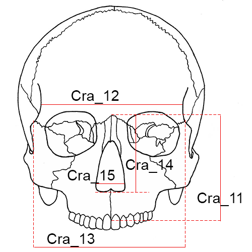
Cra_11 Nasion-Prosthion Height (n-pr, NPH): The distance from nasion (n) to prosthion (pr), upper facial height.
- Instrument: sliding caliper
- Comment: Place the fixed point of the caliper on (n) and apply the movable point to (pr). If the alveolar process exhibits slight resorption or erosion at the point of (pr), the projection of the process may be estimated when the alveolar process of the lateral incisors is still intact. When resorption or erosion is more pronounced, this measurement should not be taken (Howells 1973:174; Moore-Jansen et al. 1994, #10; Langley et al. 2016:66-67, #11).
Cra_12 Minimum Frontal Breadth (ft-ft, WFB): The distance between the right and left frontotemporale (ft).
- Instrument: sliding caliper
- Comment: Place the skull on its base. The two endpoints of the caliper are placed on the temporal ridges at the two (ft). When taking this measurement make certain that the least distance between both temporal lines on the frontal bone is recorded (Hrdlicka 1920: 15; Martin and Knussmann 1988:170, #9; Moore-Jansen et al. 1994, #11; Langley et al. 2016:67, #12).
Cra_13 Upper Facial Breadth (fmt-fmt): The distance between the right and left frontomalare temporale (fmt).
- Instrument: sliding caliper
- Comment: The measurement is taken between the two external points on the frontomalar suture (Martin and Knussmann 1988:179, #43; Moore-Jansen et al. 1994, #12; Langley et al. 2016:67, #13).
Cra_14 Nasal Height (n-ns, NLH): The average height from nasion (n) to the lowest point on the border of the nasal aperture on either side (ns).
- Instrument: sliding caliper
- Comment: Place the skull on its occiput, base to the right, and measure the distance from (n) to the inferior border of the nasal aperture on each side and take the average of these two measurements to the nearest whole millimeter. The lower border of the aperture is well defined in most populations. It is not always the most anterior edge, but the beginning of the actual floor of the nasal cavity. It is the hinder border, not the forward border, of any prenasal gutter or fossa. (Howells 1973:175; Moore-Jansen et al. 1994, #13; Langley et al. 2016:67, #14).
Cra_15 Nasal Breadth (al-al, NLB): The maximum breadth of the nasal aperture (al-al).
- Instrument: sliding caliper
- Comment: Carefully place the points of the instrument on the sharp lateral margins of the nasal aperture at its most lateral curvature; this is not an inside measurement. The measurement is perpendicular to the mid-sagittal plane and recorded to the nearest millimeter (Howells 1973: 176; Martin and Knussmann 1988:181, #54; Moore-Jansen et al. 1994, #14; Langley et al. 2016:68, #15).
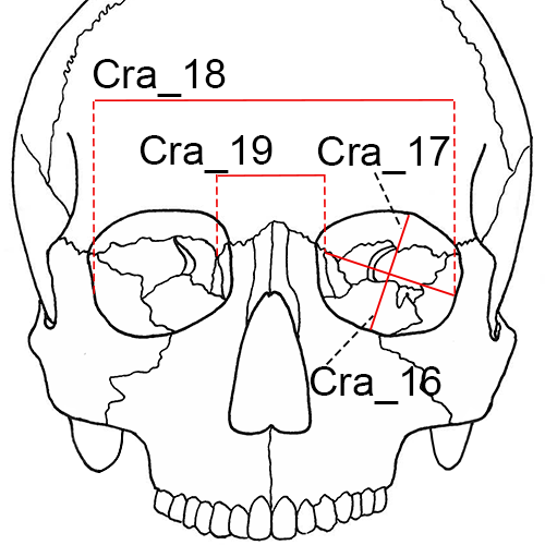
Cra_16L and Cra_16R Orbital Breadth (d-ec, OBB): The distance from dacryon (d) to ectoconchion (ec), of the left (L) and right (R) orbit, respectively.
- Instrument: sliding caliper
- Comment: The inside jaws of the calipers are useful for this measurement. For standardization and practical reasons measure the left orbit. Measure the right orbit if the left orbit is damaged and record the side measured on the recording sheet. (Howells 1973: 175; Martin and Knussmann l988:181, #51a; Moore-Jansen et al. 1994, #15; Langley et al. 2016:68, #16).
Cra_17L and Cra_17R Orbital Height (OBH): The distance between the superior and inferior orbital margins perpendicular to orbital breadth and bisecting the orbit into equal medial and lateral halves, of the left (L) and right (R) orbit, respectively.
- Instrument: sliding caliper
- Comment: Orbital height is measured perpendicular to orbital breadth. Any notches or depressions on either superior or inferior borders should be avoided; if there is deep notching, move the caliper medially slightly. The inside jaws of the calipers are useful for this measurement. (Howells 1973: 175; Martin and Knussmann 1988:181, #52; Moore-Jansen et al. 1994, #16; Langley et al. 2016:68, #17).
Cra_18 Biorbital Breadth (ec-ec, EKB): The distance from left to right ectoconchion (ec) (Howells 1973:178; Moore-Jansen et al. 1994, #17; Langley et al. 2016:68, #18).
- Instrument: sliding caliper
Cra_19 Interorbital Breadth (d-d, DKB): The distance between right and left dacryon (d) (Howells 1973:178; Moore-Jansen et al. 1994, #18; Langley et al. 2016:69, #19).
- Instrument: sliding caliper
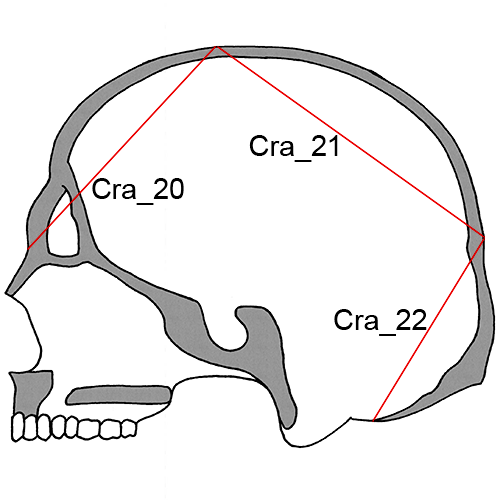
Cra_20 Frontal Chord (n-b, FRC): The distance from nasion (n) to bregma (b) taken in the mid-sagittal plane.
- Instrument: sliding caliper
- Comment: Place the tips of the instrument on the bone surface or at the level of the bone surface and not in a suture or other depression (Howells 1973:181; Martin and Knussmann 1988:174, #29; Moore-Jansen et al. 1994, #19; Langley et al. 2016:69, #20).
Cra_21 Parietal Chord (b-l, PAC): The distance from bregma (b) to lambda (l) taken in the mid-sagittal plane.
- Instrument: sliding caliper
- Comment: Place the tips of the instrument on the bone surface or at the level of the bone surface and not in a suture or other depression (Howells 1973:182; Martin and Knussmann 1988:175, #30; Moore-Jansen et al. 1994, #20; Langley et al. 2016:69, #21).
Cra_22 Occipital Chord (l-o, OCC): The distance from lambda (l) to opisthion (o) taken in the mid-sagittal plane (Howells 1973:182; Martin and Knussmann 1988:175, #31; Moore-Jansen et al. 1994, #21; Langley et al. 2016:69, #22).
- Instrument: sliding caliper
Cra_23 Foramen Magnum Length (ba-o, FOL): The mid-sagittal distance from the most anterior point on the foramen magnum margin to opisthion (o).
- Instrument: sliding caliper
- Comment: Measure with the skull base up, using the inside jaws of the calipers (Martin and Knussmann 1988:169 #7; Moore-Jansen et al. 1994, #22; Langley et al. 2016:69, #23).
Cra_24 Foramen Magnum Breadth (FOB): The distance between the lateral margins of the foramen magnum at the point of greatest lateral curvature.
- Instrument: sliding caliper
- Comment: Measure with the skull base up using the inside jaws of the calipers (Martin and Knussmann 1988:171, #16; Moore-Jansen et al. 1994, #23; Langley et al. 2016:69, #24).
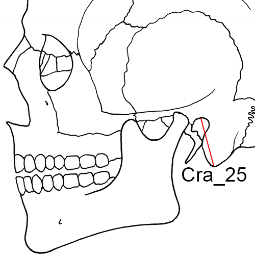
Cra_25L and Cra_25R Mastoid Height (MDH): The direct distance between porion (po) and mastoidale (ms) of the left (L) and right (R) sides, respectively.
- Instrument: sliding caliper
- Comment: Note that both right and left sides are measured. Place the fixed arm of the caliper on (po) and move the movable arm until it touches (ms). This may be most easily accomplished by holding the calipers in a coronal plane. Howells (1973:176) and Martin and Knussmann (1988:172, #19a) define this measurement similarly, though their measurement technique differs from that described here. When only one value is needed, average the right and left measurements. If the discrepancy between the sides is more than 2 mm, repeat as a check (Moore-Jansen et al. 1994, #24; Langley et al. 2016:69-70, #25).
Cra_26 Biasterionic Breadth (ast-ast, ASB): The straight-line distance from left to right asterion (ast).
- Instrument: sliding caliper
- Comment: With the skull resting so that the occiput is facing the observer, measure the distance using the sharp points of the calipers (Howells 1973:174; Martin and Knussmann 1988:171, #12; Langley et al. 2016:70, #26).
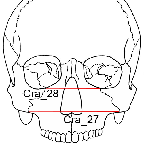
Cra_27 Bimaxillary Breadth (zma-zma, ZMB): The breadth across the maxillae, from the left to right zygomaxillare anterior (zma).
- Instrument: sliding caliper
- Comment: The endpoints of the measurement are located on the facial surface and not on the inferior aspect of the zygomaxillary suture (Howells 1973:177; Langley et al. 2016:70, #27).
Cra_28 Zygoorbitale Breadth (zo-zo, ZOB): The distance between right and left zygoorbitale (zo) (Langley et al. 2016: 70, #28).
- Instrument: sliding caliper
Mandible
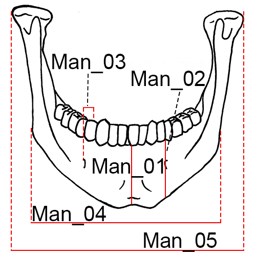
Mandible, anterior view.
Man_01 Chin Height (id-gn): The distance from infradentale (id) to gnathion (gn).
- Instrument: sliding caliper
- Comment: When the mandibular alveolar process is damaged between the central incisors, estimates of this measurement are recorded by using the intact alveolar process at the position of the lateral incisors. Any estimate or adjustment should be indicated on the recording form. In mandibles where the alveolar process exhibit pronounced erosion or resorption, this measurement is not taken (Martin and Knussmann 1988:183, #69; Moore-Jansen et al. 1994, #25; Langley et al. 2016:71, #29).
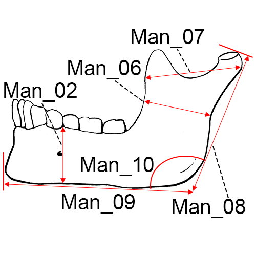
Mandible, lateral left view.
Man_02L and Man_02R Height of the Mandibular Body: The distance from the alveolar process to the inferior border of the mandible at the level of the mental foramen (Martin and Knussmann 1988:183, #69.1; Moore-Jansen et al. 1994, #26; Langley et al. 2016:71, #30), of the left (L) and right (R) sides, respectively.
- Instrument: sliding caliper
Man_03L and Man_03R Breadth of the Mandibular Body: The maximum breadth measured at the level of the mental foramen perpendicular to the long axis of the mandibular body (Martin and Knussmann 1988:183, #69.3; Moore-Jansen et al. 1994, #27; Langley et al. 2016:71, #31), of the left (L) and right (R) sides, respectively.
- Instrument: sliding caliper
Man_04 Bigonial Breadth (go-go): The distance between the right and left gonion (go).
- Instrument: sliding caliper
- Comment: Apply the blunt points of the caliper arms to the most prominent external points at the mandibular angles (Martin and Knussmann 1988:182, #66; Moore-Jansen et al. 1994, #28; Langley et al. 2016:71, #32).
Man_05 Bicondylar Breadth (cdl-cdl): The distance between the most lateral points on the mandibular condyles (cdl).
- Instrument: sliding caliper
- Comment: Place the blunt point of the fixed end of the instrument against the right condyle and apply the movable end to the left condyle (Martin and Knussmann 1988:182, #65; Moore-Jansen et al. 1994, #29; Langley et al. 2016:71, #33).
Man_06L and Man_06R Minimum Ramus Breadth: The minimum breadth of the mandibular ramus measured perpendicular to the height of the ramus, of the left (L) and right (R) sides, respectively.
- Instrument: sliding caliper
- Comment: The measurement is taken at the waist of the ramus (the point where the distance between the anterior and posterior margins of the ramus is the smallest) (Martin and Knussmann 1988:183, #71a; Moore-Jansen et al. 1994, #30; Langley et al. 2016:72, #34).
Man_07L and Man_07R Maximum Ramus Breadth: Distance between the most anterior point on the mandibular ramus and a line connecting the most posterior point on the condyle and the angle of the jaw (Moore-Jansen et al. 1994, #31), of the left (L) and right (R) sides, respectively.
- Instrument: sliding caliper
Man_08 Maximum Ramus Height: The distance from gonion (go) to the highest point on the mandibular condyle.
- Instrument: mandibulometer
- Comment: Apply movable board of the mandibulometer to the posterior borders of the mandibular rami and the fixed board against the most anterior point of the chin (Martin and Knussmann 1988:183, #70; Moore-Jansen et al. 1994, #32; Langley et al. 2016:72, #35).
Man_09 Mandibular Length: The distance from the anterior margin of the chin to the midpoint of a straight line extending from the posterior border of the right and left mandibular angles (Martin and Knussmann 1988:182, #68; Moore-Jansen et al. 1994, #33; Langley et al. 2016:72, #36).
- Instrument: mandibulometer
Man_10 Mandibular Angle: The angle formed by inferior border of the corpus and the posterior border of the ramus.
- Instrument: mandibulometer
- Comment: In case of “rocker jaws”, the bone is held in place by pressing down on the second molars (Martin and Knussmann 1988:185, #79; Moore-Jansen et al. 1994, #34; Langley et al. 2016:72, #37).
Man_11 Mandibular Body Breadth at the Mental Foramen: The maximum width of the mandibular body taken at the mental foramen.
- Instrument: sliding caliper
- Comment: The measurement is typically taken from a superior-to-interior direction and the caliper arm should be parallel to the flat surface on which the mandible is resting (Berg 2014, TML).
Man_12 Mandibular Body Breadth at the M2/M3 Junction: The maximum mediolateral breadth of the corpus taken at the level of the articulation between the second and third molars.
- Instrument: sliding caliper
- Comment: The sliding caliper arm should be parallel to the surface upon which the mandible rests. The measurement location usually corresponds to a medial-lateral thickening of the mandible at that location (Berg 2014, TML23).
Man_13 Dental Arcade Width at the Third Molar: The maximum breadth of the dental arcade at the level of the most posterior points of the third molar crypt on the lingual surface.
- Instrument: sliding caliper
- Comment: If necessary, a line should be drawn perpendicular to the ramus body and the tooth crypt to mark the measurement locations. If the third molars are absent, the measurement could be taken at the location of the second molar position, but should be annotated appropriately (Berg 2014, XDA).
Vertebrae
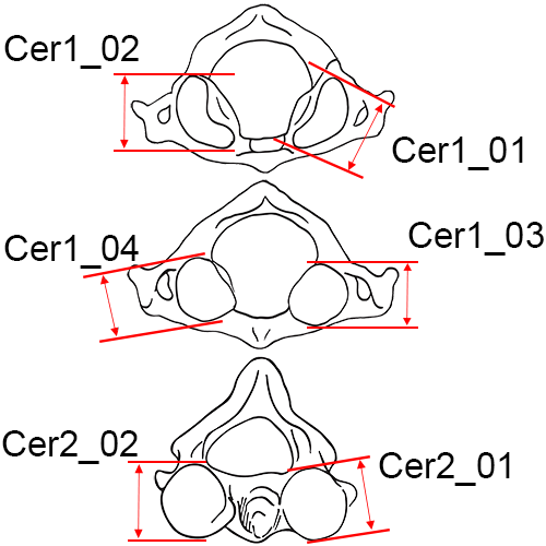
Cer1_01 (Left) and Cer1_02 (Right) Maximum Length of the Superior Articular Facet of C1: Take the maximum length of the facet as it appears in any direction (Byrd and Adams 2015, #81A).
- Instrument: sliding caliper
Cer1_03 (Left) and Cer1_04 (Right) Maximum Length of the Inferior Articular Facet of C1: Take the maximum length of the facet as it appears in any direction (Byrd and Adams 2015, #81M).
- Instrument: sliding caliper
Cer2_01 (Left) and Cer2_02 (Right) Maximum Length of the Superior Articular Facet of C2: Take the maximum length of the facet as it appears in any direction (Byrd and Adams 2015, #81B).
- Instrument: sliding caliper
Clavicle
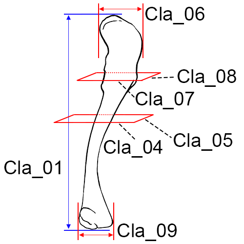
Left clavicle, inferior view.
Cla_01 Maximum Length of the Clavicle: The maximum distance between the most extreme ends of the clavicle.
- Instrument: osteometric board
- Comment: Place the bone on the osteometric board and place the sternal end of the clavicle against the vertical end board. Press the movable upright against the acromial end and move the bone up, down and sideways until the maximum length is obtained (Martin and Knussmann 1988:197, #1; Moore-Jansen et al. 1994, #35; Langley et al. 2016:73, #38).
Cla_02 Maximum Diameter of the Clavicle at Midshaft: The maximum diameter of the bone measured at midshaft.
- Instrument: sliding caliper
- Comment: Determine the midpoint of the diaphysis on the osteometric board and mark it with a pencil. Place the bone between the two arms of the caliper and rotate the bone until the maximum diameter is obtained (Langley et al. 2016:73, #39).
Cla_03 Minimum Diameter of the Clavicle at Midshaft: The minimum diameter of the bone measured at midshaft.
- Instrument: sliding caliper
- Comment: Determine the midpoint of the diaphysis on the osteometric board and mark it with a pencil. Place the bone between the two arms of the caliper and rotate the bone until the minimum diameter is obtained (Langley et al. 2016:74, #40).
Cla_04 Sagittal (Anterior-Posterior) Diameter at Midshaft: The distance from the anterior to the posterior surface at midshaft.
- Instrument: sliding caliper
- Comment: Determine the midpoint of the diaphysis on the osteometric board and mark it with a pencil. Then determine sagittal diameter (Martin 1957:528, #5; Moore-Jansen et al. 1994, #36).
Cla_05 Vertical (Superior-Inferior) Diameter at Midshaft: The distance from the superior to the inferior surface at midshaft.
- Instrument: sliding caliper
- Comment: Taken perpendicular to sagittal diameter (Martin 1957:528, #1; Moore-Jansen et al. 1994, #37).
Cla_06 Maximum Width at the Distal End: The maximum width of the distal end of the clavicle where the calipers are in contact with the rough attachment area, taken perpendicular to the shaft. Avoid angling the calipers (Byrd and Adams 2015, #37A).
- Instrument: sliding caliper
Cla_07 Breadth at the Inflexion Point at the Distal End: Anchor the caliper in the concave curve of the inflexion point at the distal end of the clavicle and place the other jaw of the caliper on the opposite side usually on or near the tubercle (Byrd and Adams 2015, #37B).
- Instrument: sliding caliper
Cla_08 Maximum Thickness at the Inflexion Point at the Distal End: The maximum thickness in the same vertical plane as the previous measurement (take perpendicular to breadth at the inflection point measurement) (Byrd and Adams 2015, #37C).
- Instrument: sliding caliper
Cla_09 Maximum Anterior-Posterior Width at the Proximal End: The maximum anterior-posterior width of the proximal end (be sure to hold in anatomical position) (Byrd and Adams 2015, #37D).
- Instrument: sliding caliper
Scapula
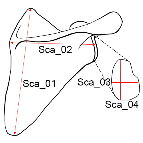
Right scapula, posterior view.
Sca_01 Height of the Scapula (Anatomical Height): The distance from the most superior point of the cranial angle to the most interior point on the caudal angle (Martin and Knussmann 1988:197, #1; Moore-Jansen et al. 1994, #38; Langley et al. 2016:74, #41).
- Instrument: sliding caliper or osteometric board
Sca_02 Breadth of the Scapula (Anatomical Breadth): The distance from the midpoint on the dorsal border of the glenoid fossa to midway between the two ridges of the scapular spine on the vertebral border.
- Instrument: sliding or spreading calipers
- Comment: Project a line through the obtuse angle of a triangle formed by the vertebral border and the two ridges of the spine, dividing it into two equal halves. The medial measuring point is located where this line intersects the vertebral border (Hrdlicka 1920:131; Moore-Jansen et al. 1994, #39; Langley et al. 2016:74, #42).
Sca_03 Glenoid Cavity Breadth: Maximum distance from the ventral to dorsal margins (anterior/posterior) of the glenoid cavity, taken perpendicular to glenoid cavity height. In cases of severe lipping, this measurement should not be taken (Martin and Knussmann 1988:198, #13, Langley et al. 2016:74, #43).
- Instrument: sliding caliper
- Comment: Place one flat surface of the jaw of the calipers on the anterior side of the glenoid fossa and place the flat surface of the other jaw on the posterior side with both jaws oriented parallel to the long axis of the bone (Byrd and Adams 2015, #39B).
Sca_04 Glenoid Cavity Height: The distance from the most superiorly located point on the margin of the glenoid cavity to the most inferiorly located point on the margin, taken perpendicular to glenoid cavity breadth. Often a distinct rim is visible (look at the fossa from the side and take the measurement at the apex of the ridges). In cases of severe lipping, this measurement should not be taken (Martin and Knussmann 1988: 198, #12; Langley et al. 2016: 74, #44; Byrd and Adams 2015, #39A).
- Instrument: sliding caliper
Sca_05 Minimum Length from Scapular Notch to Axillary Border: This measurement is the minimum distance from the superior border (typically in the notch) to the axillary border. Anchor a jaw of the caliper in the notch and use the other jaw to find the minimum distance to a point on the axillary border (Byrd and Adams 2015, #39D).
- Instrument: sliding caliper
Humerus
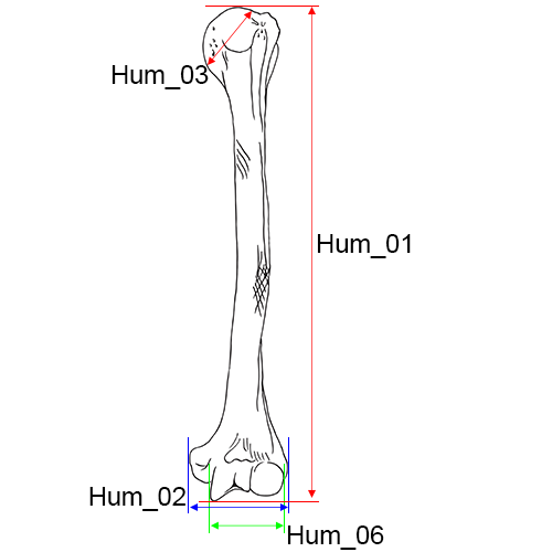
Right humerus, anterior view.
Hum_01 Maximum Length of the Humerus: The distance from the most superior point on the head of the humerus to the most inferior point on the trochlea.
- Instrument: osteometric board
- Comment: Place the humerus on the osteometric board so that its long axis parallels theinstrument. Place the head of the humerus against the vertical end board and press the movable upright against the trochlea. Move the bone up, down and sideways to determine the maximum distance (Hrdlicka 1920:126; Moore-Jansen et al. 1994, #40; Langley et al. 2016:74, #45).
Hum_02 Epicondylar Breadth of the Humerus: The distance from the most laterally protruding point on the lateral epicondyle to the corresponding projection on the medial epicondyle (Martin and Knussmann 1988:199, #4; Moore-Jansen et al. 1994, #41; Langley et al. 2016:74, #46).
- Instrument: osteometric board or sliding caliper
Hum_03 Maximum Vertical Diameter of Head: The distance between the most superior and inferior points on the border of the articular surface.
- Instrument: sliding caliper
- Comment: Do not include arthritic lipping which may be present on the perimeter of the joint surface. This diameter is not necessarily the maximum head diameter (Martin and Knussmann 1988:200, #10; Moore-Jansen et al. 1994, #42; Langley et al. 2016:74, #47).
Hum_04 Maximum Diameter of the Humerus at Midshaft: The maximum diameter of the humeral shaft at midshaft.
- Instrument: sliding caliper
- Comment: Determine the midpoint of the diaphysis on the osteometric board and mark with a pencil. Using sliding calipers to measure with one hand, rotate the bone with the other hand until the maximum diameter is obtained. (Martin and Knussmann 1988:199, #5; Moore-Jansen et al. 1994, #43; Langley et al. 2016:74-75, #48).
Hum_05 Minimum Diameter of the Humerus at Midshaft: The minimum diameter of the humeral shaft at midshaft.
- Instrument: sliding caliper
- Comment: Determine the midpoint of the diaphysis on the osteometric board and mark with a pencil. Using sliding calipers to measure with one hand, rotate the bone with the other hand until the minimum diameter is obtained. (Martin and Knussmann 1988:199, #6; Moore-Jansen et al. 1994, #44; Langley et al. 2016:75, #49).
Hum_06 Total Breadth of the Capitulum-Trochlea: The breadth of the capitulum and trochlea at the distal humerus. One end of the sliding calipers is positioned parallel to the flat, spool-shaped surface of the trochlea (medial), and the other end is moved until it comes into contact with the capitulum (lateral) (Byrd and Adams 2003, #41A).
- Instrument: sliding caliper
Hum_07 Anterior-Posterior Breadth of the Head: The maximum breadth of the humeral head taken in the anterior-posterior direction on the articular surface. This measurement is taken perpendicular from the vertical diameter of the humeral head (Byrd and Adams 2003, #42A).
- Instrument: sliding caliper
Hum_08 Minimum Diameter of the Diaphysis: The minimum diameter of the humeral diaphysis taken in any direction perpendicular to the shaft. This measurement should be taken on the oval part of the shaft, superior to the flattening observed around the olecranon fossa and the lateral supracondylar ridge. Often it is found near midshaft (Byrd and Adams 2003, #44B).
- Instrument: sliding caliper
Hum_09 Maximum Diameter of Diaphysis at the Deltoid Tuberosity: The maximum diameter of the diaphysis within the length of the deltoid tuberosity. Rotate and slide the element to find the maximum diameter (Byrd and Adams 2015, #44D).
- Instrument: sliding caliper
Radius
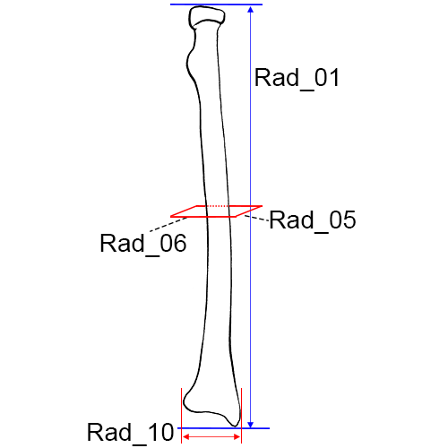
Left radius, anterior view.
Rad_01 Maximum Length of the Radius: The distance from the most proximally positioned point on the head of the radius to the tip of the styloid process without regard to the long axis of the bone.
- Instrument: osteometric board
- Comment: Place the proximal end against the vertical upright of the osteometric board and press the movable upright against the distal end. Move the bone up, down and sideways to obtain the maximum length (Martin and Knussmann 1988:201, #1; Hrdlicka 1920:127; Moore-Jansen et al. 1994, #45; Langley et al. 2016:75, #50).
Rad_02 Maximum Diameter of the Radius at Midshaft: The maximum diameter of the radial shaft taken at midshaft.
- Instrument: sliding caliper
- Comment: Mark the midshaft of the bone with a pencil. Using sliding calipers to measure with one hand, rotate the bone with the other hand until the minimum diameter is obtained (Langley et al. 2016:75, #51).
Rad_03 Minimum Diameter of the Radius at Midshaft: The minimum diameter of the radial shaft taken at midshaft.
- Instrument: sliding caliper
- Comment: Mark the midshaft of the bone with a pencil. Using sliding calipers to measure with one hand, rotate the bone with the other hand until the minimum diameter is obtained (Langley et al. 2016:75, #52).
Rad_04 Maximum Diameter of the Head: The maximum diameter of the radial head measured on the margin of the head that articulates with the ulna. The bone is rotated until the maximum distance is obtained (Montagu 1960:68; Langley et al. 2016:75, #53; Byrd and Adams 2003, #47D).
- Instrument: sliding caliper
Rad_05 Sagittal (Anterior-Posterior) Diameter at Midshaft: The distance between anterior and posterior surfaces at midshaft.
- Instrument: sliding caliper
- Comment: Determine the midpoint of the diaphysis on the osteometric board and mark with a pencil. Measure sagittal diameter at that point. This measurement is almost always less than the medial-lateral diameter (Moore-Jansen et al. 1994, #46).
Rad_06 Transverse (Medial-Lateral) Diameter at Midshaft: The distance between medial and lateral surfaces at midshaft.
- Instrument: sliding caliper
- Comment: Perpendicular to anterior-posterior diameter (Moore-Jansen et al. 1994, #47).
Rad_07 Maximum Diameter at the Radial Tuberosity: The maximum shaft diameter on the radial tuberosity. Position the calipers around the tuberosity and rotate the bone until the maximum distance is obtained (Byrd and Adams 2003, #47A).
- Instrument: sliding caliper
Rad_08 Maximum Diameter of the Diaphysis Distal to the Radial Tuberosity: The maximum shaft diameter distal to the radial tuberosity, positioned along the interosseous crest. The bone should be rotated to find the maximum distance (Byrd and Adams 2003, #47B).
- Instrument: sliding caliper
Rad_09 Minimum Diameter of the Diaphysis Distal to the Radial Tuberosity: The minimum shaft diameter anywhere distal to the radial tuberosity. The bone may be rotated to find the minimum distance (Byrd and Adams 2003, #47C).
- Instrument: sliding caliper
Rad_10 Breadth of the Distal Epiphysis: The maximum distance from the ulnar notch to the lateral aspect of the styloid process. The medial protrusions (articular borders of the ulnar notch) are placed against the vertical endboard of the osteometric board (sliding calipers may also be used) and the movable portion is applied to the lateral surface of the styloid process to find the maximum breadth (Byrd and Adams 2015, #47E).
- Instrument: sliding caliper
Ulna
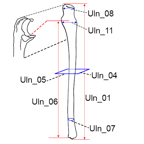
Right ulna, anterior view.
Uln_01 Maximum Length of the Ulna: The distance between the most proximal point on the olecranon and the most distal point on the styloid process.
- Instrument: osteometric board
- Comment: Place the proximal end of the ulna against the vertical end board. Press the movable upright against the distal end while moving the bone up, down and sideways to obtain the maximum length (Hrdlicka 1920:127; Martin and Knussmann 1988:204, #1; Moore-Jansen et al. 1994, #48; Langley et al. 2016:75-76, #54).
Uln_02 Maximum Midshaft Diameter of the Ulna: The maximum diameter of the diaphysis at midshaft.
- Instrument: sliding caliper
- Comment: Mark the midshaft of the bone with a pencil. Using sliding calipers to measure with one hand, rotate the bone with the other hand until the maximum diameter is obtained (Langley et al. 2016:76, #55).
Uln_03 Minimum Midshaft Diameter of the Ulna: The minimum diameter of the diaphysis at midshaft.
- Instrument: sliding caliper
- Comment: Mark the midshaft of the bone with a pencil. Using sliding calipers to measure with one hand, rotate the bone with the other hand until the minimum diameter is obtained (Langley et al. 2016:76, #56).
Uln_04 Dorso-Volar (Anterior-Posterior) Diameter: The maximum diameter of the diaphysis where the crest exhibits the greatest development in the anterior-posterior (dorso-volar) plane (Moore-Jansen et al. 1994, #49).
- Instrument: sliding caliper
Uln_05 Transverse (Medial-Lateral) Diameter: The distance between medial and lateral surfaces at the level of greatest crest development.
- Instrument: sliding caliper
- Comment: Taken perpendicular to anterior-posterior diameter (Moore-Jansen et al. 1994, #50).
Uln_06 Physiological Length of the Ulna: The distance between the deepest point on the articular surfaceof the coronoid process on the guiding ridge and the most inferior point on the distal articular surface of the ulna.
- Instrument: spreading caliper
- Comment: Do not include the styloid process or the groove between the styloid process and the distal articular surface (Martin and Knussmann 1988:204, #2; Moore-Jansen et al. 1994, #51).
Uln_07 Minimum Circumference of the Ulna: The least circumference near the distal end of the bone (Martin and Knussmann 1988:204, #3; Moore-Jansen et al. 1994, #52; Langley et al. 2016:76, #58).
- Instrument: tape
Uln_08 Olecranon Breadth: The maximum breadth of the olecranon process, taken perpendicular to the longitudinal axis of the semilunar notch (Martin and Knussmann 1988:206, #6; Langley et al. 2016:76, #59).
- Instrument: sliding caliper
Uln_09 Minimum Diameter of the Diaphysis including Interosseous Crest: Locate the minimum diameter of the diaphysis along the portion of the bone that includes the interosseous crest. This measurement may not necessarily include the interosseous crest, but should be taken on that part of the shaft that exhibits the crest. This measurement is not always near the distal end of the crest (Byrd and Adams 2003, #51A).
- Instrument: sliding caliper
Uln_10 Minimum Diameter of the Diaphysis: This measurement will be found near the distal epiphysis of the ulna. The bone should be rotated in order to locate the minimum distance (Byrd and Adams 2003, #51B).
- Instrument: sliding caliper
Uln_11 Breadth of the Semilunar Notch: This is a measure of only the distal surface of the semilunar notch (the base).
- Instrument: sliding caliper
- Comment: In order to obtain the distance, one end of the calipers is positioned within the radial notch (approximate midpoint), roughly parallel to the shaft. The other end of the calipers is applied to the medial edge of the semilunar notch to obtain the maximum distance. Calipers can be angled (Byrd and Adams 2003, #51C).
Uln_12 Physiological Length (2016): The distance between the deepest point on the articular surface of the coronoid process on the guiding ridge and the most inferior point on the distal articular surface of the ulna.
- Instrument: spreading caliper
- Comment: Do not include the styloid process or the groove between the styloid process and the distal articular surface (Langley et al. 2016:76, #57). This is an update to the Physiological Length measurement definition in Moore-Jansen et al.'s 1994 publication (measurement, #51).
Wrist and Hand
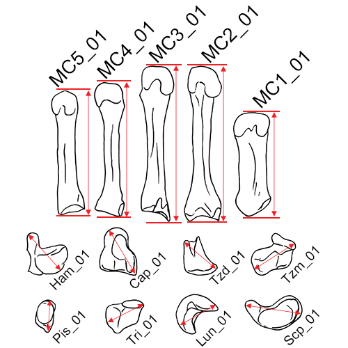
Maximum lengths of the carpals: This is the maximum length of the bone.
- Scp_01 Maximum Length of the Scaphoid (Byrd and Adams 2015, #52.5F)
- Lun_01 Maximum Length of the Lunate (Byrd and Adams 2015, #52.5G)
- Tri_01 Maximum Length of the Triquetral (Byrd and Adams 2015, #52.5H)
- Pis_01 Maximum Length of the Pisiform (Byrd and Adams 2015, #52.5I)
- Tzm_01 Maximum Length of the Trapezium (Byrd and Adams 2015, #52.5J)
- Tzd_01 Maximum Length of the Trapezoid (Byrd and Adams 2015, #52.5K)
- Cap_01 Maximum Length of the Capitate (Byrd and Adams 2015, #52.5L)
- Ham_01 Maximum Length of the Hamate (Byrd and Adams 2015, #52.5M)
Instrument: sliding caliper
Comment: Move the bone up, down, and sideways in order to obtain the maximum distance.
Maximum Lengths of the Metacarpals: This is the maximum length of the bone.
- MC1_01 Maximum Length of the 1st Metacarpal (Byrd and Adams 2015, #52.5A)
- MC2_01 Maximum Length of the 2nd Metacarpal (Byrd and Adams 2015, #52.5B)
- MC3_01 Maximum Length of the 3rd Metacarpal (Byrd and Adams 2015, #52.5C)
- MC4_01 Maximum Length of the 4th Metacarpal (Byrd and Adams 2015, #52.5D)
- MC5_01 Maximum Length of the 5th Metacarpal (Byrd and Adams 2015, #52.5E)
Instrument: sliding caliper
Comment: Move the bone up, down, and sideways in order to obtain the maximum distance.
Midline Lengths of the Metacarpals: The length from the midline of the proximal articular surface to the midline of the distal articular surface.
- MC1_02 Midline Length of the 1st Metacarpal (Meadows and Jantz 1992)
- MC2_02 Midline Length of the 2nd Metacarpal (Meadows and Jantz 1992)
- MC3_02 Midline Length of the 3rd Metacarpal (Meadows and Jantz 1992)
- MC4_02 Midline Length of the 4th Metacarpal (Meadows and Jantz 1992)
- MC5_02 Midline Length of the 5th Metacarpal (Meadows and Jantz 1992)
Instrument: sliding caliper
Sacrum
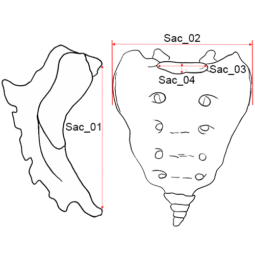
Sacrum, anterior view.
Sac_01 Anterior Height of the Sacrum: The distance from the point on the promontory in the mid-sagittal plane to the corresponding point on the anterior border of the distal tip of the sacrum.
- Instrument: sliding caliper
- Comment: Place the pointed tips of the caliper on the promontory and the anterior inferior border of the fifth sacral vertebra. The measurement is taken in the mid- sagittal plane. If a sacrum exhibits more than five segments, measure to the bottom segment and indicate the number of segments on the recording form. If the coccyx is fused to the sacrum do not include in the measurement. (Martin and Knussmann 1988:195, #2; Moore-Jansen et al. 1994, #53; Langley et al. 2016:76, #60).
Sac_02 Anterior Breadth of the Sacrum: The maximum transverse breadth of the sacrum at most anterior projection of the auricular surfaces (Martin and Knussmann 1988:195, #5; Moore-Jansen et al. 1994, #54; Langley et al. 2016:76, #61).
- Instrument: sliding caliper
Sac_03 Transverse Diameter of Sacral Segment 1: The distance between the two most lateral points on the superior articular surface measured perpendicular to the mid-sagittal plane (Martin and Knussmann 1988:195, #19).
- Instrument: sliding caliper
- Comment: The measurement should be taken on the superior articular surface of S1. When lipping of the articular surface is present approximate the original articular borders. This measurement is perpendicular to the AP Diameter of S1 (Moore-Jansen et al. 1994, #55; Langley et al. 2016:77, #62).
Sac_04 Anterior-Posterior Diameter of Sacral Segment 1: The distance between the anterior and posterior borders of the superior articular surface of S1, taken in the mid-sagittal plane (Martin and Knussmann 1988:195, #18).
- Instrument: sliding caliper
- Comment: The measurement should be taken on the superior articular surface of S1. When lipping of the articular surface is present approximate the original articular borders. This measurement is perpendicular to the Transverse Diameter of S1 (Langley et al. 2016:77, #63).
Sac_05 Maximum Breadth with the Osteometric Board: Position the sacrum on the osteometric board and find the maximum breadth of the alae (Byrd and Adams 2015, #55J).
- Instrument: osteometric board
Os coxa
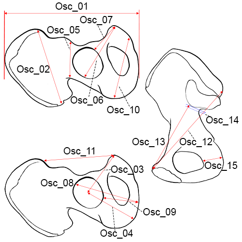
Right os coxa. Left above and below: lateral view; right: medial view.
Osc_01 Maximum Innominate Height: The distance from the most superior point on the iliac crest to the most inferior point on the ischial tuberosity (Martin and Knussmann 1988:213, #1).
- Instrument: osteometric board or spreading caliper
- Comment: When using an osteometric board, place the ischium against the vertical end board and press the movable upright against the iliac crest. Move the ilium sideways and up and down to obtain the maximum distance (Hrdlicka 1920:135; Moore-Jansen et al. 1994, #56; Langley et al. 2016:77, #64).
Osc_02 Maximum Iliac Breadth: The distance from the anterior superior iliac spine to the posterior superior iliac spine (Martin and Knussmann 1988:213, #2; Moore-Jansen et al. 1994, #57; Langley et al. 2016:77, #65).
- Instrument: spreading caliper
Osc_03 Pubis Length: The distance from the point in the acetabulum where the three elements of the os coxae meet to the upper end of the pubic symphysis.
- Instrument: sliding caliper
- Comment: The measuring point in the acetabulum may be identified in the adult by (1) an irregularity which is frequently visible, both on the acetabular and pelvic surfaces; (2) a change in thickness which may be seen by holding the bone up to a light; (3) a notch often present in the border of the articular surface in the acetabulum. In measuring the pubis, care should be taken to hold the caliper parallel to the long axis of the bone (Moore-Jansen et al. 1994, #58).
Osc_04 Ischium Length: The measuring point in the acetabulum is defined under Pubis Length. The distance from the point in the acetabulum where the three elements meet to the deepest point on the ischial tuberosity.
- Instrument: sliding caliper
- Comment: Ischium length should be measured approximately perpendicular to pubis length (Moore-Jansen et al. 1994, #59).
Osc_05 Minimum Iliac Breadth (WIB): The minimum distance measured from the area below the anterior inferior iliac spine to the most inward curvature of the greater sciatic notch (Langley et al. 2016:77, #66; Byrd and Adams 2015, #59D).
- Instrument: sliding caliper
Osc_06 Maximum Pubis Length (XPL): The distance between symphysion (the most superior point on the symphyseal face) to the farthest point on the acetabular rim.
- Instrument: spreading caliper
- Comment: The measurement is taken to the rim itself (not inside or outside the rim) (Langley et al. 2016:77, #67).
Osc_07 Minimum Pubis Length (WPL): The distance between symphysion (the most superior point on the symphyseal face) to the closest point on the acetabular rim.
- Instrument: spreading caliper
- Comment: The measurement is taken to the rim itself (not inside or outside the rim) (Langley et al. 2016:77, #68).
Osc_08 Ischial Length (ISL): The distance from the point on the acetabular rim where the iliac blade meets the acetabulum to the most medial point on the epiphysis of the ischial tuberosity.
- Instrument: sliding caliper
- Comment: If the borders of the epiphysis cannot be determined, do not take this measurement (Langley et al. 2016:77, #69).
Osc_09 Minimum Ischial Length (WISL): The distance from the most medial point on the epiphysis of the ischial tuberosity to the closest point on the acetabular rim.
- Instrument: sliding caliper
- Comment: If the borders of the epiphysis cannot be determined, do not take this measurement (Langley et al. 2016:78, #70).
Osc_10 Maximum Ischiopubic Ramus Length (XIRL): The distance from the most inferior point on the symphyseal face to the most distant point on the ischial tuberosity (Langley et al. 2016:78, #71).
- Instrument: sliding caliper
Osc_11 Anterior Superior Iliac Spine to Symphysion (ASISS): The measurement from the apex of the anterior superior iliac spine (most projecting area or point) to symphysion (Langley et al. 2016:78, #72).
- Instrument: sliding caliper
Osc_12 Maximum Posterior Superior Iliac Spine to Symphysion (PSISS): The maximum measurement from the posterior border of the posterior superior iliac spine to symphysion (Langley et al. 2016:78, #73).
- Instrument: sliding caliper
Osc_13 Maximum Apical Border to Symphysion (WAS): The minimum measurement from symphysion to the apex (anterior border) of the auricular surface (Langley et al. 2016:78, #74).
- Instrument: sliding caliper
Osc_14 Thickness of the Ilium at the Sciatic Notch: Position one end of the calipers along the arcuate line, adjacent to the apex of the auricular surface. Slide the opposing end of the calipers to the posterior surface of the ilium to obtain the measurement (Byrd 2008, #59A).
- Instrument: sliding caliper
Osc_15 Maximum Breadth of the Ischium: Position one end of the calipers in the obturator foramen and place the other end on the ischial tuberosity. Move the calipers around to find the maximum distance (Byrd and Adams 2015, #59B).
- Instrument: sliding caliper
Osc_16 Minimum Breadth of the Pubis: Position the calipers along the iliopubic ramus; rotate and slide the calipers to find the minimum distance. Use the pointed edges of the calipers instead of the flat so as not to obstruct the measurement (Byrd and Adams 2015, #59C).
- Instrument: sliding caliper
Osc_17 Maximum Diameter of the Acetabulum: The maximum distance of the acetabulum taken at any two points along the articular border of the lunate surface (look at the acetabulum from the side and take the measurement at the peaks of the ridges). This distance is commonly found in line with the iliac crest and the ischial tuberosity (Byrd 2008, #59E).
- Instrument: sliding caliper
Femur
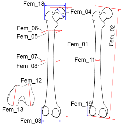
Left femur, posterior view.
Fem_01 Maximum Length of the Femur: The distance from the most proximal point on the head of the femur to the most distal point on the medial or lateral femoral condyle (Martin and Knussmann 1988:216, #1).
- Instrument: osteometric board
- Comment: Place the femur parallel to the long axis of the osteometric board and resting on its posterior surface. Press the medial or lateral condyle against the vertical end board while applying the movable upright to the femoral head. Move the bone up, down, and sideways until the maximum length is obtained (Hrdlicka 1920:128; Moore-Jansen et al. 1994, #60; Langley et al. 2016:78, #75).
Fem_02 Bicondylar Length of the Femur: The distance from the most proximal point on the head of the femur to a plane drawn between the inferior surfaces of the distal condyles.
- Instrument: osteometric board
- Comment: Place the femur on the osteometric board so that the bone is resting on its posterior surface. Press both distal condyles against the vertical end board while applying the movable upright to the head of the femur (Hrdlicka 1920:128; Martin and Knussmann 1988:216, #2; Moore-Jansen et al. 1994, #61; Langley et al. 2016:78, #76).
Fem_03 Epicondylar Breadth of the Femur: The distance between the two most projecting points on the epicondyles.
- Instrument: osteometric board
- Comment: Place the femur on the osteometric board so that it is resting on its posterior surface. Press one of the epicondyles against the vertical end board while applying the movable upright to the other condyle. (Martin and Knussmann 1988:218, #21; Moore-Jansen et al. 1994, #63; Langley et al. 2016:79, #77).
Fem_04 Maximum Diameter of the Femur Head: The maximum diameter of the femur head measured on the border of the articular surface.
- Instrument: sliding caliper
- Comment: Rotate the arms of the caliper around the femur head to find the maximum diameter. (Dwight 1905:21; Montagu 1960:70; Moore-Jansen et al. 1994, #63; Langley et al. 2016:79, #78).
Fem_05 Medial-Lateral (Transverse) Subtrochanteric Diameter of the Femur: The transverse diameter of the proximal portion of the diaphysis at the point of its greatest lateral expansion.
- Instrument: sliding caliper
- Comment: The transverse diameter is oriented parallel to the anterior surface of the femur neck. Close attention should be paid to assessing this plane in femoral necks with a significant degree of torsion. In cases where this cannot be determined (e.g. where the lateral surfaces remain parallel) this measurement is recorded in the region 2-5 cm below the lesser trochanter (Martin and Knussman 1988:217, #9; Moore-Jansen et al. 1994, #65; Langley et al. 2016:79-80, #79).
Fem_06 Anterior-Posterior (Sagittal) Subtrochanteric Diameter of the Femur: The anterior-posterior diameter of the proximal end of the diaphysis measured perpendicular to the transverse diameter at the point of the greatest lateral expansion (See definition Fem_05 for approximate location on the femoral shaft for this measurement). This diameter is oriented perpendicular to the anterior surface of the femur neck (Martin and Knussman 1988:217, #10; Moore-Jansen et al. 1994, #64; Langley et al. 2016:80, #80).
- Instrument: sliding caliper
Fem_07 Anterior-Posterior (Sagittal) Midshaft Diameter: The distance between anterior and posterior surfaces measured approximately at the midpoint of the diaphysis, at the highest elevation of linea aspera.
- Instrument: sliding caliper
- Comment: The sagittal diameter should be measured perpendicular to the anterior bone surface (Moore-Jansen et al. 1994, #66).
Fem_08 Medial-Lateral (Transverse) Midshaft Diameter: The distance between the medial and lateral surfaces at midshaft, measured perpendicular to the anterior-posterior diameter (Moore-Jansen et al. 1994, #67).
- Instrument: sliding caliper
Fem_09 Maximum Midshaft Diameter of the Femur: The maximum diameter of the femoral shaft taken at midshaft.
- Instrument: sliding caliper
- Comment: Mark the midshaft of the bone with a pencil. Using sliding calipers to measure with one hand, rotate the bone with the other hand until the maximum diameter is obtained (Langley et al. 2016:80, #81).
Fem_10 Minimum Midshaft Diameter of the Femur: The minimum diameter of the femoral shaft taken at midshaft.
- Instrument: sliding caliper
- Comment: Mark the midshaft of the bone with a pencil. Using sliding calipers to measure with one hand, rotate the bone with the other hand until the minimum diameter is obtained (Langley et al. 2016:80, #82).
Fem_11 Circumference of the Femur at Midshaft: The circumference measured at the midshaft.
- Instrument: tape
- Comment: If the linea aspera is unusually hypertrophied at midshaft, this measurement should be recorded approximately 10 mm above the midshaft (Martin and Knussmann 1988:217, #8; Moore-Jansen et al. 1994, #68; Langley et al. 2016:80, #83).
Fem_12 Maximum Anterio-posterior Length of the Lateral Condyle: The distance between the most anterior and posterior points on the articular surface of the lateral condyle (Martin and Knussman 1988:219, #23).
- Instrument: sliding caliper
- Comment: Holding the femur with the distal end up, orient the measuring arms of the caliper with the long axis of the bone to obtain this measurement (Langley et al. 2016:80, #84).
Fem_13 Maximum Anterio-posterior Length of the Medial Condyle: The distance between the most anterior and posterior points on the articular surface of the medial condyle (Martin and Knussman 1988:219, #24).
- Instrument: sliding caliper
- Comment: Holding the femur with the distal end up, orient the measuring arms of the caliper with the long axis of the bone to obtain this measurement (Langley et al. 2016:80-81, #85).
Fem_14 Minimum Anterior-Posterior Diameter of the Diaphysis: The minimum anterior-posterior diameter anywhere along the diaphysis. The linea aspera and condyles should be utilized in order to orient the bone in anatomical position (use the condyles to orient) (Byrd and Adams 2003, #68A).
- Instrument: sliding caliper
Fem_15 Minimum Medial-Lateral Diameter of the Diaphysis: The minimum medial-lateral diameter anywhere along the diaphysis. The linea aspera and condyles should be utilized in order to orient the bone (should be taken in a perpendicular orientation to 68A) (Byrd and Adams 2003, #68B).
- Instrument: sliding caliper
Fem_16 Minimum Superior-Inferior Neck Diameter: The minimum distance from the superior surface to the inferior surface on the femoral neck (Seidemann et al. 1998). Place caliper in the saddle of the neck (superior) and close inferior caliper arm, moving as necessary to find the minimum (Byrd and Adams 2015, #68D).
- Instrument: sliding caliper
Fem_17 Maximum Diameter along the Linea Aspera: The maximum shaft diameter at any point along the linea aspera. As the bone should be rotated to obtain the maximum distance, the measurement does not necessarily have to include the linea aspera, though it likely will (Byrd and Adams 2003, #68E).
- Instrument: sliding caliper
Fem_18 Upper Breadth of Femur (VHA): The distance from the apex of the head of the femur to the lateral side of the femur diaphysis, measured in line with the neck of the femur such that the line of measurement bisects the neck. Using sliding calipers, place the fixed jaw on the most prominent point on the femur head. Place the movable jaw on the lateral margin of the femur diaphysis so that the line formed between the two points splits the neck into two equal portions (Simmons et al. 1990).
- Instrument: sliding caliper
Fem_19 Lateral Condyle Height (LCH): On the lateral condyle of the distal femur, it is the distance from the most superior point on the condyle to the most inferior point. Holding the femur in anatomical position with the distal condyles facing the observer, place the fixed jaw of the sliding caliper on the top of the condyle and place the movable jaw on the most inferior point on the condyle. The femur should be held so that it is possible to accurately judge the location of the most inferior point (Simmons et al. 1990).
- Instrument: sliding caliper
Patella
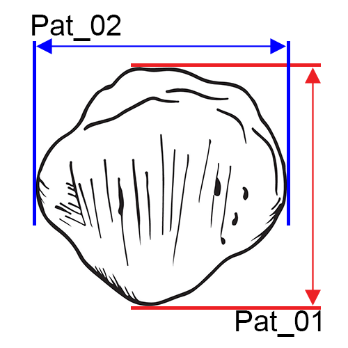
Pat_01 Maximum Length of the Patella: Find the maximum length (superior to inferior) of the patella (Byrd and Adams 2015, #74.5A).
- Instrument: sliding caliper
Pat_02 Maximum Breadth: Find the maximum breadth (medial to lateral) of the patella (Byrd and Adams 2015, #74.5B).
- Instrument: sliding caliper
Pat_03 Maximum Thickness: Find the maximum thickness (anterior to posterior) of the patella (Byrd and Adams 2015, #74.5C).
- Instrument: sliding caliper
Tibia
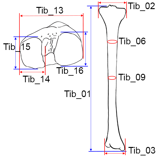
Left tibia, anterior view.
Tib_01 Length of the Tibia: The distance from the superior articular surface of the lateral condyle of the tibia to the tip of the medial malleolus (Martin and Knussmann 1988:220, #1).
- Instrument: osteometric board
- Comment: An osteometric board with a hole for the intercondylar eminence makes this measurement easier to take. Place the tibia on the osteometric board resting on its posterior surface with the longitudinal axis of the bone parallel to the board (Hrdlicka 1920:129). If using an osteometric board without a hole, place the tibia on the osteometric board so that it the long axis is parallel to the board. The measurement is taken from the lateral condyle to the tip of the medial malleolus (Moore-Jansen et al. 1994, #69; Langley et al. 2016:81, #86).
Tib_02 Maximum Proximal Epiphyseal Breadth of the Tibia: The maximum distance between the two most projecting point on the margins of the medial and lateral condyles of the proximal epiphysis.
- Instrument: osteometric board
- Comment: Place the tibia on the osteometric board resting on its posterior surface. Press the lateral condyle against the vertical end board, and place the movable upright against the medial condyle. Tibiae exhibiting marked torsion may have to be rotated to obtain the maximum breadth (Martin and Knussmann 1988:221, #3; Moore-Jansen et al. 1994, #70; Langley et al. 2016:81, #87).
Tib_03 Maximum Distal Epiphyseal Breadth: The distance between the most medial point on the medial malleolus and the lateral surface of the distal epiphysis.
- Instrument: osteometric board
- Comment: Place the two lateral protrusions of the distal epiphysis against the fixed side of the osteometric board and move the sliding board until it contacts the medial malleolus (Martin and Knussmann 1988:221, #6; Moore-Jansen et al. 1994, #71; Langley et al. 2016:81, #88).
Tib_04 Maximum Diameter at the Nutrient Foramen: The distance between the anterior crest and the posterior surface at the level of the nutrient foramen (Moore-Jansen et al. 1994, #72).
- Instrument: sliding caliper
Tib_05 Transverse (Medial-Lateral) Diameter at the Nutrient Foramen: The straight line distance from the medial margin to the interosseous crest at the level of the nutrient foramen (Moore-Jansen et al. 1994, #73).
- Instrument: sliding caliper
- Comment: This is taken perpendicular to Maximum Diameter at the Nutrient Foramen.
Tib_06 Circumference at the Nutrient Foramen: The circumference measured at the level of the nutrient foramen (Moore-Jansen et al. 1994, #74).
- Instrument: tape
Tib_07 Maximum Midshaft Diameter of the Tibia: The maximum diameter of the tibial shaft taken at midshaft.
- Instrument: sliding caliper
- Comment: Mark the midshaft of the bone with a pencil. Using sliding calipers to measure with one hand, rotate the bone with the other hand until the maximum diameter is obtained (Langley et al. 2016:81, #89).
Tib_08 Minimum Midshaft Diameter of the Tibia: The minimum diameter of the tibial shaft taken at midshaft.
- Instrument: sliding caliper
- Comment: Mark the midshaft of the bone with a pencil. Using sliding calipers to measure with one hand, rotate the bone with the other hand until the minimum diameter is obtained (Martin and Knussmann 1988:573, #9a; Langley et al. 2016:81, #90).
Tib_09 Circumference of the Tibia at the Midshaft: The circumference measured at the level of the midshaft (Martin and Knussmann 1988:574, #10a; Langley et al. 2016:82, #91).
- Instrument: tape
Tib_10 Maximum Anterior-Posterior Diameter Distal to the Popliteal Line: This measurement should be taken at the most distal point of the popliteal line where it intersects with the margin of the diaphysis. The calipers are rotated to find the maximum distance (this is the maximum diameter of the diaphysis at this point). Note that the correct location may be difficult to determine in very gracile individuals (Byrd and Adams 2003, #74A).
- Instrument: sliding caliper
Tib_11 Minimum Anterior-Posterior Diameter: Locate the minimum anterior-posterior distance at any point on the tibial shaft. Use the medial malleolus and anterior crest to orient the bone, particularly when torsion is present (Byrd and Adams 2003, #74B).
- Instrument: sliding caliper
Tib_12 Maximum Anterior-Posterior Distance of the Distal Articular Surface: Locate the maximum anterior-posterior distance of the distal articular surface by viewing the element from the side to find the peaks of the articular surface and measuring the distance between them. Use the medial malleolus to orient the bone (Byrd and Adams 2015, #74F).
- Instrument: sliding caliper
Tib_13 Biarticular Breadth (BB): Maximum breadth of the proximal articular surface of the tibia as measured from the lateral edge of the lateral condyle to the medial edge of the medial condyle. This is not the maximum breadth of the proximal tibia, but rather the maximum breadth of the articular surface. Holding the tibia so that the proximal articular surface is in plain view, place the fixed jaw of the digital caliper on the most lateral edge of the lateral condyle. Extend the movable jaw to what appears to be the most medial edge of the medial condyle. Pivot the movable jaw slightly to ensure that the maximum measure is found (Holland 1992).
- Instrument: sliding caliper
Tib_14 Medial Condyle Articular Width (MCW): Maximum transverse width of the medial condyle as measured from lateral to medial edges. The surface of the condyle generally is circumscribed by a slight rim, and points of the caliper should be placed on this rim. Hold the tibia so that you can look directly down on the proximal articular surface. Place the fixed jaw of the digital caliper on the medial edge of the condyle. Extend the movable jaw to the lateral edge of the medial condyle. Move the caliper anteriorly and then posteriorly, adjusting the jaws so that they always contact the opposing edges of the condyle. Find the maximum in this manner (Holland 1992).
- Instrument: sliding caliper
Tib_15 Medial Condyle Articular Length (MCL): Similar but perpendicular to width. Measurement should record maximum length from the anterior edge of the medial condyle to the posterior margin. Hold the tibia so that you can look directly down on the proximal articular surface. Place the fixed jaw of the digital caliper on the anterior edge of the medial condyle. Extend the movable jaw to the posterior edge of the condyle. Move the caliper medially and then laterally, adjusting the jaws so that they always contact the opposing edges of the condyle. Find the maximum in this manner (Holland 1992).
- Instrument: sliding caliper
Tib_16 Lateral Condyle Articular Length (LCL): Maximum length of the lateral condyle as measured in a manner similar to that for MCL (Holland 1992).
- Instrument: sliding caliper
Fibula
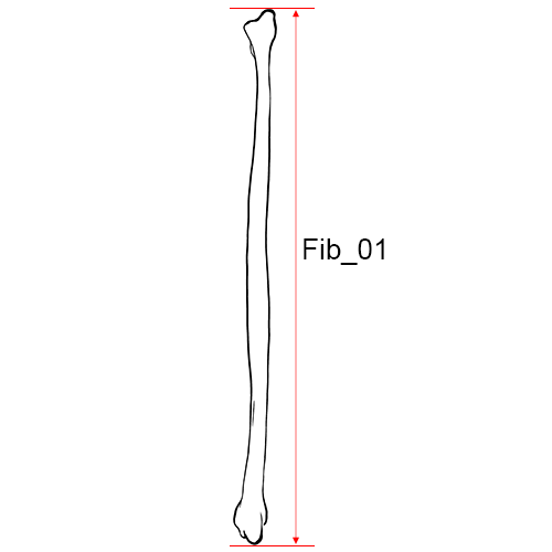
Left fibula, anterior view.
Fib_01 Maximum Length of the Fibula: The maximum distance between the most superior point on the fibular head and the most inferior point on the lateral malleolus (Martin and Knussmann 1988:222, #1).
- Instrument: osteometric board
- Comment: Place the fibula on the osteometric board and place the tip of the lateral malleolus against the vertical end board. Press the movable upright against the proximal end of the bone while moving it up and down and sideways to obtain the maximum length (Moore-Jansen et al. 1994, #75; Langley et al. 2016:82, #92).
Fib_02 Maximum Diameter of the Fibula at Midshaft: The maximum diameter at the midshaft. (Martin and Knussmann 1988:222, #2).
- Instrument: sliding caliper
- Comment: Find the midpoint on the osteometric board and mark with a pencil. Place the diaphysis of the fibula between the two arms of the caliper while turning the bone to obtain the maximum diameter (Moore-Jansen et al. 1994, #76; Langley et al. 2016:82, #93).
Fib_03 Maximum Diameter of the Diaphysis: This measurement should only be taken along the interosseous crest. Avoid measurements of the shaft near the epiphyses (Byrd and Adams 2015, #76A).
- Instrument: sliding caliper
Fib_04 Minimum Diameter of the Diaphysis: The minimum distance at any point along the diaphysis (Byrd and Adams 2015, #76B).
- Instrument: sliding caliper
Fib_05 Maximum Breadth at the Distal End: Place the one jaw of the caliper on the posterior portion (tubercle) and extend the other jaw to the opposite side (just above the malleolar articular surface) to find the maximum distance (Byrd and Adams 2015, #76C).
- Instrument: sliding caliper
Ankle and foot
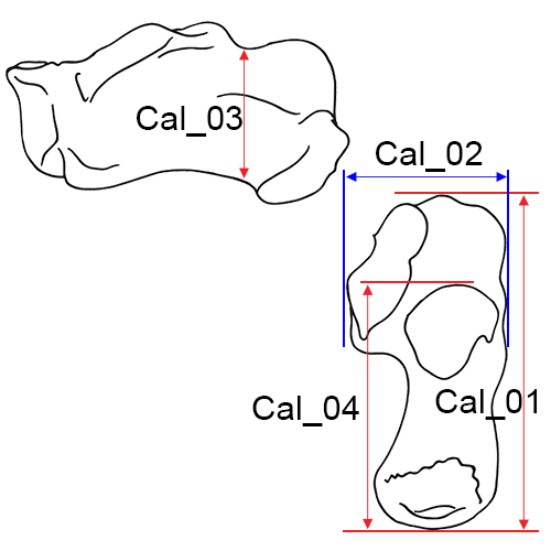
Cal_01 Maximum Length of the Calcaneus (MCAL): The distance between the most posteriorly projecting point on the calcaneal tuberosity and the most anterior point on the superior margin of the articular facet for the cuboid measured in the sagittal plane (Martin and Knussmann 1988:225 #1).
- Instrument: sliding caliper or osteometric board
- Comment: Excessive calcaneal spurs should be omitted from this measurement (Moore-Jansen et al. 1994, #77; Holland 1995, MCAL; Langley et al. 2016:82, #94).
Cal_02 Middle Breadth of the Calcaneus: The distance between the most laterally projecting point on the dorsal articular facet and the most medial point on the sustentaculum tali.
- Instrument: sliding caliper
- Comment: The two measuring points lie at neither the same level, nor in a plane perpendicular to the sagittal plane. Span the calcaneus from behind with the blunt arms of the caliper so that the caliper is positioned in a flat and transverse plane across the bone (Martin and Knussmann 1988:225, #2; Moore-Jansen et al. 1994, #78; Langley et al. 2016:82, #95).
Cal_03 Minimum Height Distal to Articular Facets: Find the minimum height in the pinched area of the calcaneus distal to the articular facets and proximal to the calcaneal tuber (Byrd and Adams 2015, #78A).
- Instrument: sliding caliper
Cal_04 Posterior Length of the Calcaneus (PCAL): Maximum length between the most anterior point of the posterior talar articular surface and the most posterior point of the calcaneus (on the tuberosity ignoring any extensive exostoses). Hold the calcaneus in anatomical position so that you are looking down on the articular surface. Place the fixed jaw of the calipers on the posterior margin of the talar articular surface and extend the movable jaw to the posterior surface of the bone. Move the calipers slightly up and down and medially and laterally to find the maximum. Avoid any exostoses (Holland 1995; Byrd and Adams 2015, #78B).
- Instrument: sliding caliper
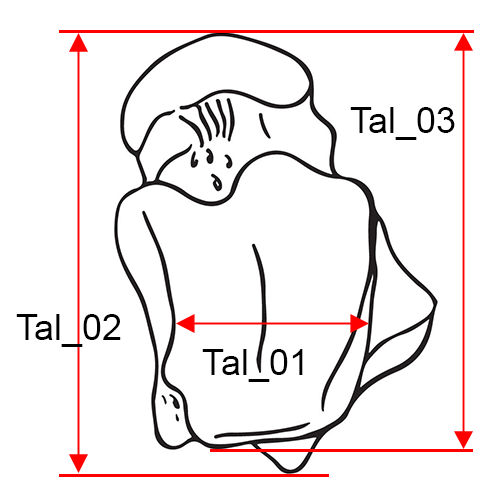
Tal_01 Minimum Trochlear Breadth: This is the minimum breadth of the trochlea (superior articular surface). Place the flat surfaces of the jaws of the sliding calipers on either side of the articular surface with the jaws (approximately) parallel to the long axis of the bones. Close the jaws to take the minimum value (Byrd 2008, #79).
- Instrument: sliding caliper
Tal_02 Maximum Length of the Talus (MTAL): The maximum length between the most anterior point of the head and the posterior tubercle (Holland, 1995; Byrd and Adams 2015, #79A).
- Instrument: sliding caliper
Tal_03 Maximum Articular Length: The maximum length between the most anterior point of the head and the posterior surface of the tibial articulation (excluding the tubercle). Position the fixed caliper arm along the posterior surface of the tibial articulation and bring the calipers closed on the most anterior point of the head (Byrd and Adams 2015, #79B).
- Instrument: sliding caliper
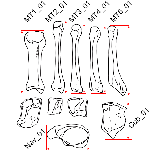
Maximum Lengths of the Tarsals: This is the maximum length of the bone.
- Cub_01 Maximum Length of the Cuboid (Byrd and Adams 2015, #80F)
- Nav_01 Maximum Length of the Navicular (Byrd and Adams 2015, #80G)
- Cf1_01 Maximum Length of the 1st Cuneiform (Byrd and Adams 2015, #80H)
- Cf2_01 Maximum Length of the 2nd Cuneiform (Byrd and Adams 2015, #80I)
- Cf3_01 Maximum Length of the 3rd Cuneiform (Byrd and Adams 2015, #80J)
Instrument: sliding caliper
Comment: Move the bone up, down, and sideways in order to obtain the maximum distance, in the same manner that maximum length is obtained for the humerus, femur, etc.
Maximum Lengths of the Metatarsals: This is the maximum length of the bone.
- MT1_01 Maximum Length of the 1st Metatarsal (Byrd and Adams 2015, #80A)
- MT2_01 Maximum Length of the 2nd Metatarsal (Byrd and Adams 2015, #80B)
- MT3_01 Maximum Length of the 3rd Metatarsal (Byrd and Adams 2015, #80C)
- MT4_01 Maximum Length of the 4th Metatarsal (Byrd and Adams 2015, #80D)
- MT5_01 Maximum Length of the 5th Metatarsal (Byrd and Adams 2015, #80E)
Instrument: osteometric board or sliding caliper
Comment: Move the bone up, down, and sideways in order to obtain the maximum distance, in the same manner that maximum length is obtained for the humerus, femur, etc.
Measurement Standards Table
The measurement standards table can be downloaded here, was originally provided by OsteoCodeR.com. Please visit OsteoCodeR below for more information.
The standardized measurements table is provided below for your reference.
| OsteoSort | S1994 | UTK1994 | UTK2016 | BA2003 |
|---|---|---|---|---|
| Cla_01 | 35 | 35 | 38 | |
| Cla_02 | 39 | |||
| Cla_03 | 40 | |||
| Cla_04 | 36 | 36 | ||
| Cla_05 | 37 | 37 | ||
| Cla_06 | 37A | |||
| Cla_07 | 37B | |||
| Cla_08 | 37C | |||
| Cla_09 | 37D | |||
| Sca_01 | 38 | 38 | 41 | |
| Sca_02 | 39 | 39 | 42 | |
| Sca_03 | 43 | 39B | ||
| Sca_04 | 44 | 39A | ||
| Sca_05 | 39D | |||
| Hum_01 | 40 | 40 | 45 | |
| Hum_02 | 41 | 41 | 46 | |
| Hum_03 | 42 | 42 | 47 | |
| Hum_04 | 43 | 43 | 48 | |
| Hum_05 | 44 | 44 | 49 | |
| Hum_06 | 41A | |||
| Hum_07 | 42A | |||
| Hum_08 | 44B | |||
| Hum_09 | 44D | |||
| Rad_01 | 45 | 45 | 50 | |
| Rad_02 | 51 | |||
| Rad_03 | 52 | |||
| Rad_04 | 53 | 47D | ||
| Rad_05 | 46 | 46 | ||
| Rad_06 | 47 | 47 | ||
| Rad_07 | 47A | |||
| Rad_08 | 47B | |||
| Rad_09 | 47C | |||
| Rad_10 | 47E | |||
| Uln_01 | 48 | 48 | 54 | |
| Uln_02 | 55 | |||
| Uln_03 | 56 | |||
| Uln_04 | 49 | 49 | ||
| Uln_05 | 50 | 50 | ||
| Uln_06 | 51 | 51 | ||
| Uln_07 | 52 | 52 | 58 | |
| Uln_08 | 59 | |||
| Uln_09 | 51A | |||
| Uln_10 | 51B | |||
| Uln_11 | 51C | |||
| Uln_12 | 57 | |||
| Sac_01 | 53 | 53 | 60 | |
| Sac_02 | 54 | 54 | 61 | |
| Sac_03 | 55 | 55 | 62 | |
| Sac_04 | 63 | |||
| Sac_05 | 55J | |||
| Osc_01 | 56 | 56 | 64 | |
| Osc_02 | 57 | 57 | 65 | |
| Osc_03 | 58 | 58 | ||
| Osc_04 | 59 | 59 | ||
| Osc_05 | 66 | 59D | ||
| Osc_06 | 67 | |||
| Osc_07 | 68 | |||
| Osc_08 | 69 | |||
| Osc_09 | 70 | |||
| Osc_10 | 71 | |||
| Osc_11 | 72 | |||
| Osc_12 | 73 | |||
| Osc_13 | 74 | |||
| Osc_14 | 59A | |||
| Osc_15 | 59B | |||
| Osc_16 | 59C | |||
| Osc_17 | 59E | |||
| Fem_01 | 60 | 60 | 75 | |
| Fem_02 | 61 | 61 | 76 | |
| Fem_03 | 62 | 62 | 77 | |
| Fem_04 | 63 | 63 | 78 | |
| Fem_05 | 65 | 65 | 79 | |
| Fem_06 | 64 | 64 | 80 | |
| Fem_07 | 66 | 66 | ||
| Fem_08 | 67 | 67 | ||
| Fem_09 | 81 | |||
| Fem_10 | 82 | |||
| Fem_11 | 68 | 68 | 83 | |
| Fem_12 | 84 | |||
| Fem_13 | 85 | |||
| Fem_14 | 68A | |||
| Fem_15 | 68B | |||
| Fem_16 | 68D | |||
| Fem_17 | 68E | |||
| Tib_01 | 69 | 69 | 86 | |
| Tib_02 | 70 | 70 | 87 | |
| Tib_03 | 71 | 71 | 88 | |
| Tib_04 | 72 | 72 | ||
| Tib_05 | 73 | 73 | ||
| Tib_06 | 74 | 74 | ||
| Tib_07 | 89 | |||
| Tib_08 | 90 | |||
| Tib_09 | 91 | |||
| Tib_10 | 74A | |||
| Tib_11 | 74B | |||
| Tib_12 | 74F | |||
| Fib_01 | 75 | 75 | 92 | |
| Fib_02 | 76 | 76 | 93 | |
| Fib_03 | 76A | |||
| Fib_04 | 76B | |||
| Fib_05 | 76C | |||
| Cal_01 | 77 | 77 | 94 | |
| Cal_02 | 78 | 78 | 95 | |
| Cal_03 | 78A | |||
| Cal_04 | 78B | |||
| Pat_01 | 74.5A | |||
| Pat_02 | 74.5B | |||
| Pat_03 | 74.5C | |||
| Tal_01 | 79 | |||
| Tal_02 | 79A | |||
| Tal_03 | 79B | |||
| Nav_01 | 80G | |||
| Cf1_01 | 80H | |||
| Cf2_01 | 80I | |||
| Cf3_01 | 80J | |||
| Cub_01 | 80F | |||
| MT1_01 | 80A | |||
| MT2_01 | 80B | |||
| MT3_01 | 80C | |||
| MT4_01 | 80D | |||
| MT5_01 | 80E | |||
| Pis_01 | 52.5I | |||
| Scp_01 | 52.5F | |||
| Tzm_01 | 52.5J | |||
| Tzd_01 | 52.5K | |||
| Tri_01 | 52.5H | |||
| Lun_01 | 52.5G | |||
| Cap_01 | 52.5L | |||
| Ham_01 | 52.5M | |||
| MC1_01 | 52.5A | |||
| MC2_01 | 52.5B | |||
| MC3_01 | 52.5C | |||
| MC4_01 | 52.5D | |||
| MC5_01 | 52.5E |
-
Langley, N.R., L.M. Jantz, S.D Ousley, R.L. Jantz, and G. Milner (2016) Data Collection Procedures for Forensic Skeletal Material 2.0. University of Tennessee and Lincoln Memorial University ↩
Methods
In this section we present an annotated bibliography of analytical methods available in CoRA. This list will be updated as new methods are developed, published and added to the CoRA environment.
How can I add new methods to CoRA?
You can request new methods to be added to CoRA if the one you are looking for is not present by creating an issue on our issue tracker.
Sex
Bass WM (2005)
Human Osteology: A laboratory and field manual, 5th edition. Missouri Archaeological Society, Columbia, MO.
- Purpose: Sex determination from the skull.
- Characteristics of the cranium and mandible at six non-metric features are described (male vs. female): supraorbital ridge (prominent vs. smooth), supraorbital margins (blunt vs. sharp), palate/dentition (large vs. small), mastoid processes (large vs. small), frontal sinuses (large vs. small), and chin shape (square vs. rounded).
Buikstra JE, Ubelaker DH (1994)
Standards for Data Collection from Human Skeletal Remains. Arkansas Archeological Survey Research Series No. 44, Fayetteville, AR.
- Purpose: Discussion of sexually dimorphic morphology of the skull and os coxae and the association with male and female.
- CRANIAL MORPHOLOGY
- Features of the cranium and mandible are scored from minimal expression ("1") to maximal expression ("5").
- Nuchal crest: View the lateral profile of the occipital and compare it with the diagram. Feel the surface of the occipital with your hand and note any surface rugosity, ignoring the contour of the underlying bone. Focus upon the rugosity attendant to attachment of nuchal musculature. In the case of minimal expression, the external surface of the occipital is smooth with no bony projections visible when the lateral profile is viewed. Maximal expression defines a massive nuchal crest that projects a considerable distance from the bone and forms a well-defined bony ledge or "hook."
- Mastoid process: Score this feature by comparing its size with that of the surrounding structures such as the external auditory meatus and the zygomatic process of the temporal bone. The most important variable to consider in scoring this trait is the volume of the mastoid process, not its length. Minimal expression is a very small mastoid process that projects only a small distance below the inferior margins of the external auditory meatus and the digastric groove. A massive mastoid process with lengths and widths several times that of the external auditory meatus would be considered maximal expression.
- Supraorbital margin: Begin by holding your finger against the margin of the orbit at the lateral aspect of the supraorbital foramen. Then hold the edge of orbit between your fingers to determine its thickness. Look at each of the diagrams to determine which it seems to match most closely. In an example minimal expression, the border should feel extremely sharp, like the edge of a slightly dulled knife. A thick, rounded margin with a curvature approximating a pencil should be scored as maximal expression.
- Glabella: Viewing the cranium from the side. Minimal expression is characterized by minimal prominence of the glabella/supraorbital ridges with the contour of the frontal being smooth and little to no projection at the midline. Maximal expression involves a massive glabellar prominence, forming a rounded, loaf-shaped projection that is frequently associated with well-developed supraorbital ridges.
- Mental eminence: Hold the mandible between the thumbs and index fingers with thumbs on either side of the mental eminence. Move the thumbs medially until the delimit the lateral borders of the mental eminence. In examples of minimal expression, there is little or no projection of the mental eminence above the surrounding bone. By contrast, massive expression is one in which the mental eminence occupies most of the anterior portion of the mandible.
- OS COXAE MORPHOLOGY
- See Phenice (1969) for morphology/scoring of the ventral arc, subpubic concavity, and ischiopubic ramus.
- Greater sciatic notch: This feature tends to be broad in females and narrow in males. The shape of the greater sciatic notch is not as reliable as the subpubic region. For scoring this feature, it is best to use the diagrams provided in the original publication to find the closest match. The broadest notch is scored as "1", while the narrowest is scored as "5".
- Preauricular sulcus: The preauricular sulcus appears more often in females than males, with four positive expressions (score of 1-4) and the lack of expression (score of "0"). The scores are as follows: 0 = absence of preauricular sulcus; 1 = the preauricular sulcus is wide; 2 = the preauricular sulcus is wide (usually greater than 0.5 cm) but shallow; 3 = the preauricular sulcus is well defined but narrow, less than 0.5 cm deep; 4 = the preauricular sulcus is a narrow (less than 0.5 cm), shallow, and smooth-walled depression.
- OVERALL ASSESSMENT
- Based on an overall assessment of all sexually dimorphic features of the os coxae and skull, separately, an individual can be assigned:
- 0 = undetermined sex. Insufficient data are available for sex determination
- 1 = female. There is little doubt that the structures represent a female.
- 2 = probable female. The structures are more likely female than male.
- 3 = ambiguous sex. Sexually diagnostic features are ambiguous.
- 4 = probable male. The structures are most likely male than female.
- 5 = male. There is little doubt that the structures represent a male.
Phenice TW (1969)
A newly developed visual method of sexing the os pubis. American Journal of Physical Anthropology 30:297-301.
- Purpose: Sex estimation based on three features of the adult os coxa: the ventral arc, subpubic concavity, and the ischiopubic ramus.
- Sample: Terry Skeletal Collection, Smithsonian Institution; n = 275; Black and White males (n = 20 and 160, respectively) and females (n = 52 and 43, respectively).
- Each feature is determined to be: 1) female, 2) ambiguous, or 3) male.
- Ventral arc: Slightly elevated ridge extending inferiorly from pubic crest across the ventral surface to the lateral most extension of the subpubic concavity. Present in females.
- Subpubic concavity: A lateral recurve of the ischio-pubic ramus below the lower margin of the pubic symphysis. Present in females.
- Ischiopubic ramus: Portion extending from the inferior pubic symphysis to the ischial tuberosity. The ramus is broad and generally flat in males, while a narrower ramus with a ridge is typical of female morphology.
- The ischiopubic ramus is most likely to display ambiguous morphology, and the ventral arc is least likely to display ambiguous morphology.
- If sex assessment is based on one or two of the features that are definitely male or female (ventral arc and subpubic concavity), the estimate will be correct at least 96% of the time.
Rogers TL (1999)
A visual method of determining the sex of skeletal remains using the distal humerus. Journal of Forensic Sciences 44:57-60.
- Purpose: Sex estimation based on the characteristics of four dimorphic features of the distal humerus: trochlear constriction, trochlear asymmetry, olecranon fossa shape and depth, and the angle of the medial epicondyle. These are "scored" as male or female based on their morphology.
- Sample: Developed on the Grant Skeletal Collection, University of Toronto (20th century anatomy series), n = 202 (175 males, 27 females); tested on known individuals from the University of New Mexico Documented Collection (n = 35; 28 males, 7 females) and the William M. Bass Donated Skeletal Collection (n = 93; 74 males, 19 females).
- Trochlear constriction: constricted and spool-shaped in females; less constricted in males.
- Trochlear symmetry: asymmetrical in females; symmetrical in males.
- Olecranon fossa shape and depth: deep oval in females; shallow triangle in males. Shape is more important than depth.
- Angle of the medial epicondyle: distinctly raised in females; flat or slightly raised in males.
- In ambiguous cases (two traits scored as male, two traits scored as female), greater weight should be given to the olecranon fossa.
- The greatest accuracy is achieved when all four features are present and scorable.
Rogers NL, Flournoy LE, McCormick WF (2000)
The rhomboid fossa of the clavicle as a sex and age estimator. Journal of Forensic Sciences 45:61-67.
- Purpose: Sex estimation based on clavicle morphology, specifically, the presence or absence of the rhomboid fossa, which is a pitted or depressed marking on the inferior sternal end of the clavicle.
- Sample: William F. McCormick Skeletal Collection, University of Tennessee - Knoxville; n = 344; 113 females, 231 males; White (n=301), Black (n=38), "Other" non-White (n=5); Ages: 10-92 years.
- Males are more likely than females to have a rhomboid fossa, and rhomboid fossae are more commonly exhibited in younger individuals than older individuals.
- Posterior probabilities (left clavicle): fossa present, P(male) = 92.2%, P(female) = 7.8%; fossa absent, P(male) = 41.4%, P(female) = 58.6%
- Posterior probabilities (right clavicle): fossa present, P(male) = 81.7%, P(female) = 18.3%; fossa absent, P(male) = 41.0%, P(female) = 59.0%
- Authors suggest these posterior probabilities cannot be used on other populations, but due to the preponderance of fossae on male clavicles, the presence of a fossa likely indicates a male individual.
Walker PL (2005)
Greater sciatic notch morphology: Sex, age, and population differences. American Journal of Physical Anthropology 127:385-391.
- Purpose: Provides empirical probabilities of being male or female for a given sciatic notch score, following Buikstra and Ubelaker (1994).
- Sample: Americans from the Hamann-Todd Collection, Cleveland Museum of Natural History and Terry Skeletal Collection, Smithsonian Institution (n = 211; 114 males, 97 females); and Europeans from the St. Bride's Collection, St. Bride's Church in London (n = 85; 51 males, 34 females).
- A score of 1 typically indicates a female, while a score of 3 or greater usually indicates a male. A score of 2 represents intermediate morphology, although a larger percentage of males than females exhibit this degree of expression.
- Probability of being male for each score: 1 - 0.12; 2 - 0.66; 3 - 0.88; 4 - 0.93; 5 - 0.90.
- Probability of being female for each score: 1 - 0.88; 2 - 0.34; 3- 0.12; 4 - 0.07; 5 - 0.10
- There is also a relationship between age-at-death and sciatic notch score, with younger people tending to have wider greater sciatic notches.
Walker PL (2008)
Sexing skulls using discriminant function analysis of visually assessed traits. American Journal of Physical Anthropology 136:39-50.
- Purpose: Provides empirical probabilities of being male for a given score of observed cranial morphology following the ordinal scales presented in Buikstra and Ubelaker (1994).
- Sample: Americans from the Hamann-Todd Collection, Cleveland Museum of Natural History and Terry Skeletal Collection, Smithsonian Institution and Europeans from the St. Bride's Collection, St. Bride's Church in London (n = 304; 164 males, 140 females). In addition, archaeological specimens (7000 B.P. to European contact) from the Santa Barbara Museum of Natural History and the Department of Anthropology, University of California, Santa Barbara were utilized (n = 156).
- The sectioning point is 0, and scores less than 0 are more likely to be male, and scores greater than 0 are more likely to be female.
- The probability of being male for each trait for a given score is provided.
- Discriminant function equations are also provided, utilizing the scores of two to three characteristics.
Age
Albert AM, Maples WR (1995)
Stages of epiphyseal union for thoracic and lumbar vertebral centra as a method of age determination for teenage and young adult skeletons. Journal of Forensic Sciences 40:623-633.
- Purpose: Age estimation by scoring fusion of thoracic and lumbar vertebral centra. This scoring is modified from McKern and Stewart (1957).
- Sample: C.A. Pound Human Identification Laboratory, University of Florida (n = 55; 33 males, 22 females); Black and White individuals (n = 9 and 46, respectively) between the ages of 11 and 32 years.
- Scoring: Stage 0 - no union; Stage 1 - epiphysis has begun to unite or is in the process of uniting to the vertebral column; Stage 2 - epiphysis is almost completely united or shows recent complete union; Stage 3 - epiphysis is completely united to the centrum.
- 16 years and younger: Stage 0 and Stage 1 noted
- 17-20 years: all stages noted
- 21 years and older: Stage 2 and Stage 3 noted
- The correlation between stages of union and known age was 0.78 (P < .0001).
Berg GE (2008)
Pubic bone age estimation in adult women. Journal of Forensic Sciences 53:569-577.
- Purpose: Age estimation for older females, re-defining the Suchey-Brooks phases V and VI, and adding phase VII.
- Sample: n = 189 females; Balkan (n = 85) and William M. Bass Donated (WBD) Skeletal Collection (n = 104)
- The calculated mean and standard deviations for the WBD sample are listed below and can be applied to an American female population.
- Phase IV: 35.5 ± 3.8 yrs
- Phase V: 49.7 ± 5.8 yrs
- Phase VI: 64.2 ± 9.0 yrs
- Phase VII: 74.2 ± 10.9 yrs
Blankenship JA, Mincer HH, Anderson KM, Woods MA, Burton EL (2007)
Third molar development in the estimation of chronologic age in American Blacks as compared with Whites. Journal of Forensic Sciences 52:428-433.
- Purpose: Age estimation of African American populations by scoring third molar development radiographically using the Demirjian et al. stages (A-H).
- Sample: n = 637 African Americans and n = 563 American Whites, between 14.0 and 24.9 years, from across the United States and Canada. The American White sample was obtained from a previous study.
- Black–White differences were significant with developmental stages occurring in Blacks a year or so earlier than Whites.
- The empirical likelihood that an African American male with fully developed M3's is at least 18 years old is 93% and that for African American female is 84%. Corresponding risks for Whites are 90% and 93%, respectively.
Brooks S, Suchey JM (1990)
Skeletal age determination based upon the os pubis: A comparison of the Acsádi-Nemeskéri and Suchey-Brooks methods. Human Evolution 5:227-238.
- Purpose: The Suchey-Brooks system is a 6-phase system (I-VI) for age estimation for males and females that utilizes the morphology of the entire symphyseal surface following the six phase system for males described by Katz and Suchey (1986).
- Sample: n = 1,225, males and females, of known ages at death from the Los Angeles Medical Examiner’s Office.
- Phase Descriptions and Ages (mean ± 1 SD, 95% range)
- Phase I: Symphyseal face has a billowing surface (ridges and furrows) which usually extends to include the pubic tubercle. The horizontal ridges are well-marked and ventral beveling may be commencing. Although ossific nodules may occur on the upper extremity, a a key to the recognition of this phase is the lack of delimitation of either upper or lower extremity. Females: 19.4 ± 2.6 yrs (15-24 yrs); Males: 18.5 ± 2.1 yrs (15-23 yrs).
- Phase II: The symphyseal face may still show ridge development. The face has commencing delimitation of lower and/or upper extremities occurring with or without ossific nodules. The ventral rampart may be in beginning phases as an extension of the bony activity at either or both extremities. Females: 25.0 ± 4.9 yrs (19-40 yrs); Males: 23.4 ± 3.6 yrs (19-34 yrs).
- Phase III: Symphyseal face shows lower extremity and ventral rampart in process of completion. There can be a continuation of fusing ossific nodules forming the upper extremity and along the ventral border. Symphyseal face is smooth or can continue to show distinct ridges. Dorsal plateau is complete. Absence of lipping of symphyseal dorsal margin; no bony ligamentous outgrowths. Females: 30.7 ± 8.1 yrs (21-53); Males: 28.7 ± 6.5 yrs (21-46 yrs).
- Phase IV: Symphyseal face is generally fine grained although remnants of the old ridge and furrow system may still remain. Usually the oval outline is complete at this stage, but a hiatus can occur in upper ventral rim. Pubic tubercle is fully separated from the symphyseal face by definition of upper extremity. The symphyseal face may have a distinct rim. Ventrally, bony ligamentous outgrowths may occur on inferior portion of pubic bone adjacent to symphyseal face. If any lipping occurs it will be slight and located on the dorsal border. Females: 38.2 ± 10.9 yrs (26-70 yrs); Males: 35.2 ± 9.4 yrs (23-57 yrs).
- Phase V: Symphyseal face is completely rimmed with some slight depression of the face itself, relative to the rim. Moderate lipping is usually found on the dorsal border with more prominent ligamentous outgrowths on the ventral border. There is little or no rim erosion. Breakdown may occur on superior ventral border. Females: 48.1 ± 14.6 yrs (25-83 yrs); Males: 45.6 ± 10.4 yrs (27-66 yrs).
- Phase VI: Symphyseal face may show ongoing depression as rim erodes. Ventral ligamentous attachments are marked. In many individuals the pubic tubercle appears as a separate bony knob. The face may be pitted or porous, giving an appearance of disfigurement with the ongoing process of erratic ossification. Crenulations may occur. The shape of the face is often irregular at this stage. Females: 60.0 ±12.4 yrs (42-87 yrs); Males: 61.2 ± 12.2 yrs (34-86 yrs).
Buckberry JL, Chamberlain AT (2002)
Age estimation from the auricular surface of the ilium: Arevised method. American Journal of Physical Anthropology 119:231-239.
- Purpose: A composite scoring method for age estimation from the auricular surface. This method is a revision of the existing auricular surface aging method by Lovejoy et al (1985), and scores independent components of the auricular surface, rather than the gestalt.
- Sample: n = 180 known-age individuals from Christ Church, Spitalfields, London were utilized for the blind test of the new method.
- Features examined (scores): transverse organizaiton (1-5), surface texture (1-5), microporosity (1-3), macroporosity (1-3), and apical changes (1-3). After each feature is examined and scored, a composite score is generated.
- This revised method yields scores that have a higher correlation with age than the Suchey-Brooks pubic symphysis system for this sample.
- No significant differences were seen between sexes or sides; therefore, the same method and age estimates can be applied to both sexes.
- Stages (Composite Score) and Ages (mean ± 1 SD)
- Stage I (5-6): 17.33 ± 1.53 yrs (16-19 yrs)
- Stage II (7-8): 29.33 ± 6.71 yrs (21-38 yrs)
- Stage III (9-10): 37.86 ± 13.08 yrs (16-65 yrs)
- Stage IV (11-12): 51.41 ± 14.47 yrs (29-81 yrs)
- Stage V (13-14): 59.94 ± 12.95 yrs (29-88 yrs)
- Stage VI (15-16): 66.71 ± 11.88 yrs (39-91 yrs)
- Stage VII (17-19): 72.25 ± 12.73 yrs (53-92 yrs)
İşcan MY, Loth SR, Wright RK (1984)
Age estimation from the rib by phase analysis: White males. Journal of Forensic Sciences 29:1094-1104.
- Purpose: Age estimation based on the morphology of the sternal end of the fourth rib (White Males).
- Sample: n = 118 White males of known age at death from the Broward County Medical Examiner's Office, Florida.
- This system is a 9-phase system (0-8), requiring the sternal end of the 4th rib be compared to three-dimensional casts of known age exemplars.
- Phase Descriptions and Ages (mean ± 1 SD, 95% range)
- Phase 0: The articular surface is flat or billowy with a regular rim and rounded edges. The bone itself is smooth, firm, and very solid.
- Phase 1: There is a beginning amorphous indentation in the articular surface, but billowing may also still be present. The rim is rounded and regular. In some cases scallops may start to appear at the edges. The bone is still firm, smooth and solid. Mean age = 17.3 ± 0.50 yrs (16.5-18.0 yrs).
- Phase 2: The pit is now deeper and has assumed a V-shaped appearance formed by the anterior and posterior walls. The walls are thick and smooth with a scalloped or slightly wavy rim with rounded edges. The bone is firm and solid. Mean age = 21.9 ± 2.13 yrs (20.8-23.1 yrs).
- Phase 3: The deepening pit has taken on a narrow to moderately U-shape. Walls are still fairly thick with rounded edges. Some scalloping may still be present but the rim is becoming more irregular. The bone is still quite firm and solid. Mean age = 25.9 ± 3.50 yrs (24.1-27.7 yrs).
- Phase 4: Pit depth is increasing, but the shape is still a narrow to moderately wide U. The walls are thinner, but the edges remain rounded. The rim is more irregular with no uniform scalloping pattern remaining. There is some decrease in teh weight and firmness of the bone, however, the overall quality of the bone is still good. Mean age = 28.2 ± 3.83 yrs (25.7-30.6 yrs).
- Phase 5: There is little change in pit depth, but the shape in this phase is predominantly a moderately wide U. Walls show further thinning and the edges are becoming sharp. Irregularity is increasing in the rim. Scalloping pattern is completely gone and has been replaced with irregular bony projections. The condition of the bone is fairly good, however, there are some signs of deterioration with evidence of porosity and loss of density. Mean age = 38.8 ± 7.00 yrs (34.4-42.3 yrs).
- Phase 6: The pit is noticeably deep with a wide U-shape. The walls are thin with sharp edges. The rim is irregular and exhibits some rather long bony projections that are frequently more pronounced at the superior and inferior borders. The bone is noticeably lighter in weight, thinner, and more porous, especially inside the pit. Mean age = 50.0 ± 11.17 yrs (44.3-55.7 yrs).
- Phase 7: The pit is deep with a wide to very wide U-shape. The walls are thin and fragile with sharp, irregular edges and bony projections. The bone is light in weight and brittle with significant deterioration in quality and obvious porosity. Mean age = 59.2 ± 9.52 yrs (54.3-64.1 yrs).
- Phase 8: In this final phase the pit is very deep and widely U-shaped. In some cases the floor of the pit is absent or filled with bony projections. The walls are extremely thin, fragile, and brittle with sharp, highly irregular edges and bony projections. The bone is very lightweight, thin, brittle, friable, and porous. "Window" formation is sometimes seen in the walls. Mean age = 71.5 ± 10.27 yrs (65.0-78.0 yrs).
İşcan MY, Loth SR, Wright RK (1985)
Age estimation from the rib by phase analysis: White females. Journal of Forensic Sciences 30:853-863.
- Purpose: Age estimation based on themorphology of the sternal end of the fourth rib (White Females).
- Sample: The reference population consists of 86 White females of known age at death.
- This system is a 9-phase system (0-8), requiring the sternal end of the 4th rib be compared to three-dimensional casts of known age exemplars.
- Phase Descriptions and Ages (mean ± 1 SD, 95% range)
- Phase O: The articular surface is nearly flat with ridges or billowing. The outer surface of the sternal extremity of the rib is bordered by what appears to be an overlay of bone. The rim is regular with rounded edges, and the bone itself is firm, smooth, and very solid.
- Phase 1: A beginning, amorphous indentation can be seen in the articular surface. Ridges or billowing may still be present. The rim is rounded and regular with a little waviness in some cases. The bone is still solid, firm, and smooth. Mean age = 14.0 (no SD or CI provided).
- Phase 2: The pit is considerably deeper and has assumed a V-shape between the thick, smooth anterior and posterior walls. Some ridges or billowing may still remain inside the pit. The rim is wavy with some scallops beginning to form at the rounded edge. The bone itself is firm and solid. Mean age = 17.4 ± 1.52 yrs (15.5-19.3 yrs).
- Phase 3: There is only slight if any increase in pit depth, but the V-shape is wider, sometimes approaching a narrow U as the walls become a bit thinner. The still rounded edges now show a pronounced, regular scalloping pattern. At this stage, the anterior or posterior walls or both may first start to exhibit a central, semicircular arc of bone. The rib is firm and solid. Mean age = 22.6 ± 1.67 yrs (20.5-24.7 yrs).
- Phase 4: There is a noticeable increase in the depth of the pit, which now has a wide V- or narrow U-shape with, at times, flared edges. The walls are thinner but the rim remains rounded. Some scalloping is still present, along with the central arc; however, the scallops are not as well defined and the edges look somewhat worn down. The quality of the bone is fairly good but there is some decrease in density and firmness. Mean age = 27.7 ± 4.62 yrs (24.4-31.0 yrs).
- Phase 5: The depth of the pit stays about the same, but the thinning walls are flaring into a wider V- or U-shape. In most cases, a smooth, hard, plaque-like deposit lines at least part of the pit. No regular scalloping pattern remains and the edge is beginning to sharpen. The rim is becoming more irregular, but the central arc is still the most prominent projection. The bone is noticeably lighter in weight, density and firmness. The texture is somewhat brittle. Mean age = 40.0 ± 12.22 yrs (33.7-46.3 yrs).
- Phase 6: An increase in pit depth is again noted, and its V- or U-shape has widened again because of pronounced flaring at the end. The plaque-like deposit may still appear but is rougher and more porous. The walls are quite thin with sharp edges and an irregular rim. The central arc is less obvious and, in many cases, sharp points project from the rim of the sternal extremity. The bone itself is fairly thin and brittle with some signs of deterioration. Mean age = 50.7 ± 14.93 yrs (43.3-58.1 yrs).
- Phase 7: In this phase, the depth of the predominantly flared U-shaped pit not only shows no increase, but actually decreases slightly .Irregular bony growths are often seen extruding from the interior of the pit. The central arc is still present in most cases but is now accompanied by pointed projections, often at the superior and inferior borders, yet may be evidenced anywhere around the rim. The very thin walls have irregular rims with sharp edges. The bone is very light, thin, brittle, and fragile, with deterioration most noticeable inside the pit. Mean age = 65.2 ± 11.24 yrs (59.2-71.2 yrs).
- Phase 8: The floor of the U-shaped pit in this final phase is relatively shallow, badly deteriorated, or completely eroded. Sometimes it is filled with bony growths. The central arc is barely recognizable. The extremely thin, fragile walls have highly irregular rims with very sharp edges, and often fairly long projections of bone at the inferior and superior borders. "Window" formation sometimes occurs in the walls. The bone itself is in poor condition - extremely thin, light in weight, brittle, and fragile. Mean age = 76.4 ± 8.83 yrs (70.4-82.3 yrs).
Kasper KA, Austin D, Kvanli AH, Rios TR, Senn DR (2009)
Reliability of third molar development for age estimation in a Texas Hispanic population: A comparison study. Journal of Forensic Sciences 54:651-657.
- Purpose: Age estimation of Hispanic populations by scoring third molar development radiographically using the method of Demirjian et al. (1973) for crown and root formation.
- Sample: Hispanic individuals (n = 950) aged from 12-22 years
- The third molar of the Hispanic sample was found to develop 8-18 months faster than American Caucasians as reported by Mincer et al. (1993).
- Prediction intervals (95% confidence) for each stage and sex
- Maxilla
- Stage B: Females 10-21 yrs; Males 8-19 yrs
- Stage C: Females 12-18 yrs; Males 12-17 yrs
- Stage D: Females 11-19 yrs; Males 12-18 yrs
- Stage E: Females 12-20 yrs; Males 12-18 yrs
- Stage F: Females 13-20 yrs; Males 13-19 yrs
- Stage G: Females 14-21 yrs; Males 14-20 yrs
- Stage H: Females >15 yrs, with a 78.8% probability of being at least 18 years; Males >15 yrs, with a 71.4-74.7% probability of being at least 18 years
- Mandible
- Stage B: Females 11-20 yrs; Males 8-20 yrs
- Stage C: Females 12-18 yrs; Males 12-17 yrs
- Stage D: Females 11-19 yrs; Males 11-18 yrs
- Stage E: Females 13-19 yrs; Males 13-18 yrs
- Stage F: Females 14-21 yrs; Males 13-20 yrs
- Stage G: Females 14-22 yrs; Males 15-21 yrs
- Stage H: Females >16 yrs, with a 87.1-89.8% probability of being at least 18 years; Males >16 yrs, with a 85.8-86.4% probability of being at least 18 years
- Additional Reference: Demirjian A, Goldstein H, Tanner JM (1973). A new system of dental age assessment. Human Biology, 45(2):211-227.
Langley-Shirley N, Jantz RL (2010)
A Bayesian approach to age estimation in modern Americans from the clavicle. Journal of Forensic Sciences 55:571-583.
- Purpose: Age estimation based on a 3-phase or 5-phase system for medial clavicular fusion for modern American individuals.
- Sample: n = 1289 (1044 male, 245 female): 594 individuals (448 male, 146 female) between 11 and 33 years from the William F. McCormick Clavicle Collection, 354 individuals (255 male, 99 female) between 11 and 30 years from the Hamann-Todd Osteological Collection), and 341 males between 16 and 33 years from the Korean War.
- Due to secular trends, observed ages for each phase are provided separately for each sample. This information can be used to produce age ranges based on the mean and standard deviations using the most appropriate sample population.
- A Bayesian approach is also utilized to provide age ranges based on the highest posterior density of the McCormick sample for use with more modern cases. This provides a more conservative, statistically sound estimate that is less sensitive to outliers. These age ranges are provided below.
- Age ranges (95% CI) for each system and sex
- 5-phase system
- 1: Females ≤16.2 yrs; Males ≤17.4 yrs
- 2: Females 13.5-21.0 yrs; Males 14.4-23.0 yrs
- 3: Females 16.7-25.7 yrs; Males 17.9-27.5 yrs
- 4: Females 19.9-29.3 yrs; Males 20.5-30.6 yrs
- 5: Females ≥22.5 yrs; Males ≥24.1 yrs
- 3-phase system
- 1: Females ≤16.5 yrs; Males ≤17.4 yrs
- 2: Females 14.1-27.1 yrs; Males 14.9-28.5 yrs
- 3: Females ≥22.1 yrs; Males ≥24.0 yrs
Lovejoy CO, Meindl RS, Pryzbeck TR, Mensforth RP (1985)
Chronological metamorphosis of the auricular surface of the ilium: A new method for determination of adult skeletal age at death. American Journal of Physical Anthropology 68:15-28.
- Purpose: An 8-phase age estimation system based on auricular surface morphology, considering changes to the granularity and density, macroporosity, billowing, striae, apex, retroauricular area, and transverse organization.
- Sample: The Todd Collection (n = 500), the Libben Collection (n = 250), and forensic cases from the Cuyahoga County Coroner’s Office, Ohio (n = 14).
- Two completely blind tests were conducted to assess the accuracy and bias of the new method utilizing different individuals from the Todd Collection (n = 98 and 108, respectively).
- There are five basic phases in which the auricular surfaces progresses: early post-epiphyseal phase, young adult phase, mid adult phase, early senescent phase, and breakdown.
- Eight age modes are developed based on the progression of auricular surface morphology through the basic five phases. The age ranges are provided below, with the most relevant characteristics. See reference for a more detailed description for each mode.
- Age Ranges and their Relevant Characteristics
- 20-24: billowing and very fine granularity.
- 25-29: reduction of billowing, but retention of youthful appearance.
- 30-34: general loss of billowing, replacement by striae, and distinct coarsening of granularity.
- 35-39: uniform coarse granularity.
- 40-44: transition from coarse granularity to dense surface; this may take part over islands of the surface of one or both faces.
- 45-49: completion of densification with complete loss of granularity.
- 50-59: dense irregular surface of rugged topography and moderate to marked activity in periauricular areas.
- 60+: breakdown with marginal lipping, macroporosity, increased irregularity, and marked activity in periauricular areas.
Mann RW, Jantz RL, Bass WM, Willey PS (1991)
Maxillary suture obliteration: A visual method for estimating skeletal age. Journal of Forensic Sciences 36:781-791.
- Purpose: Age estimation by assessing suture closure of the four maxillary (palatal) sutures.
- Sample: 186 skeletons of known age, sex, and race from three skeletal collections (Louisiana State University, University of Tennessee, and the Terry Skeletal Collection, Smithsonian Institution): 46 White males, 32 White females, 64 Black males, and 44 Black females.
- Males exhibit more suture obliteration than females at the same age.
- Although this method cannot be used for exact estimates of individual age, it is valuable in establishing an estimated age range or minimum age.
- First Evidence of Partial Obliteration (by suture)
- Incisive: 16 yrs
- Transverse palatine: 22 yrs
- Posterior median palatine: 25 yrs
- Anterior median palatine: 27 yrs
- Earliest Complete Obliteration (by suture and sex)
- Incisive: Females 20 yrs; Males 20 yrs
- Transverse palatine: Females 27 yrs; Males 26 yrs
- Posterior median palatine: Females 84 yrs; Males 33 yrs
- Anterior median palatine: Females 67 yrs; Males 40 yrs
McKern TW, Stewart TD (1957)
Skeletal Age Changes in Young American Males. Quartermaster Research and Development Command Technical Report EP-45, Natick, MA.
- Purpose: Age estimation by scoring epiphyseal union of various skeletal elements, as well as morphology of the pubic symphysis.
- Sample: American males who died as a result of the Korean War from 1950 to 1952.
- Because this sample is represented by military males, individuals below 17 years of age are not present, and these methods are most applicable for American males who died prior to (ca.) 1960.
- Epiphyseal union: The stage of epiphyseal union is scored on a scale of 0 to 4 (0 - unfused, 1 - beginning fusion, 2 - largely fused, 3 - fused, 4 - fused with no remnant fusion line). The stage of epiphyseal fusion can then be compared to the published standards. McKern and Stewart present only raw data in tabular form.
- Pubic symphysis: The McKern-Stewart system is a 3-component system that scores the dorsal and ventral demifaces and the rim of the pubic symphysis (each component having a 0-5 stage of development). Morphology can be compared to a cast set comprised of a representative pubic symphysis for a score of 1 to 5 for each component. The scores for each component are combined and correspond to a given age range.
Meindl RS, Lovejoy CO (1985)
Ectocranial Suture Closure: a revised method for the determination of skeletal age at death based on the lateral-anterior sutures. American Journal of Physical Anthropology 68:57-66.
- Purpose: Age estimation by scoring (0-open, 1-minimal closure, 2-significant closure, 3-complete obliteration) ectocranial vault and lateral anterior suture closure at ten sites.
- Sample: Hamann-Todd Collection, Cleveland Museum of Natural History (n = 236).
- Scores are combined to produce two composite scores that correspond to estimates of age-at-death, which were found to be independent of race and sex.
Mincer HH, Harris EF, Berryman HE (1993)
The A.B.F.O. study of third molar development and its use as an estimator of chronological age. Journal of Forensic Sciences 38:379-390.
- Purpose: Age estimation for American Whites and Blacks by scoring third molar development radiographically using the eight-grade classification system by Demirjian et al. (1973).
- Sample: n = 823, males (46%) and females (54%) between the ages of 14 and 24 years from across the United States and Canada. The sample consisted of white (80%), Black (19%), and “other” (1%).
- Although the third molar is the most variable tooth, the formation of the third molar can be useful for age estimation when other elements are unavailable.
- Mean ages (± 1 SD) at attainment of stages for third molar formation
- Maxilla
- Stage D: White Females 16.0 ± 1.55 yrs; White Males 16.0 ± 1.97 yrs; Blacks nd
- Stage E: White Females 16.9 ± 1.85 yrs; White Males 16.6 ± 2.38 yrs; Blacks nd
- Stage F: White Females 18.0 ± 1.95 yrs; White Males 17.7 ± 2.28 yrs; Blacks nd
- Stage G: White Females 18.8 ± 2.27 yrs; White Males 18.2 ± 1.91 yrs; Blacks 19.3 ± 3.37 yrs
-
Stage H: White Females 20.6 ± 2.09 yrs; White Males 20.2 ± 2.09 yrs; Blacks 20.4 ± 3.14 yrs
-
Mandible
- Stage D: White Females 16.0 ± 1.64 yrs; White Males 15.5 ± 1.59 yrs; Blacks nd
- Stage E: White Females 16.9 ± 1.75 yrs; White Males 17.3 ± 2.47 yrs; Blacks nd
- Stage F: White Females 17.7 ± 1.80 yrs; White Males 17.5 ± 2.14 yrs; Blacks 17.2 ± 3.14 yrs
- Stage G: White Females 19.1 ± 2.18 yrs; White Males 18.3 ± 1.93 yrs; Blacks 18.5 ± 2.68 yrs
- Stage H: White Females 20.9 ± 2.01 yrs; White Males 20.5 ± 1.97 yrs; Blacks 21.4 ± 2.34 yrs
- If an individual has reached Stage H, then one can be reasonably confident that the individuals is at least 18 years of age. An upper age limit should not be imposed.
Nawrocki SP (1998)
Regression formulae for the estimation of age from cranial suture closure. In Forensic Osteology: Advances in the Identification of Human Remains, 2nd ed., edited by Kathy Reichs, pp. 293-317. Charles C. Thomas, Springfield, IL.
- Purpose: Age estimation by scoring ectocranial, endocranial, and maxillary suture closure.
- Sample: American White (n = 49) and Black (n = 51) males and females (n = 50 for each).
- Twenty-seven cranial landmarks are scored, including 16 from the ectocranial surface, 7 from the endocranial surface, and 4 from the palate, on a scale of 0 to 3.
- Ten of the ectocranial landmarks are the same as Meindl and Lovejoy’s (1973) landmarks.
- Scores can be summed and utilized in a regression equation to predict age.
- Eight equations for predicting age from all cranial suture landmarks are provided.
- Because incomplete crania are often recovered, additional formulae using only landmarks of the calotte are also provided (Equations 9 – 15).
Osborne DL, Simmons TL, Nawrocki SP (2004)
Reconsidering the auricular surface as an indicator of age at death. Journal of Forensic Sciences 49:905-911.
- Purpose: Age estimation based on auricular surface morphology.
- Sample: n = 266; the Terry Skeletal Collection, Smithsonian Institution (n = 72), and the Bass Donated Collection, University of Tennessee (n = 194), which represent early 20th century and late 20th century individuals, respectively.
- This method is a modified 6-phase system of the existing 8-phase auricular surface aging method by Lovejoy et al (1985).
- Phase Descriptions and Ages (mean ± 1 SD, suggested age range)
- Phase 1: Billowing with possible striae; mostly fine granularity with some coarse granularity possible. 21.1 ± 2.98 yrs (≤27 yrs)
- Phase 2: Striae; coarse granularity with residual fine granularity; retroauricular activity may be present. 29.5 ± 8.20 yrs (≤46 yrs)
- Phase 3: Decreased striae with transverse organization; coarse granularity; retroauricular activity present; beginnings of apical change. 42.0 ± 13.74 yrs (≤69yrs)
- Phase 4: Remnants of transverse organization; coarse granularity becoming replaced by densification; retroauricular activity present; apical change; macroporosity is present. 47.8 ± 13.95 yrs (20-75 yrs)
- Phase 5: Surface becomes irregular; surface texture is largely dense; moderate retroauricular activity; moderate apical change; macroporosity. 53.1 ± 14.14 yrs (24-82 yrs)
- Phase 6: Irregular surface; densification accompanied by subchondral destruction; severe retroauricular activity; severe apical change; macroporosity. 58.9 ± 15.24 yrs (29-89 yrs)
Rougé-Maillart C, Vielle B, Jousset N, Chappard D, Telmon N and Cunha E (2009)
Estimation of skeletal age at death in adults using the acetabulum and the auricular surface on a Portuguese population. Forensic science international 188(1-3), pp.91-95.
- Purpose: A composite scoring method for age estimation from a combination of the auricular surface and acetabulum.
- Sample: 462 hip bones from a series of identified skeletons, of known age and sex, from the Coimbra Identified Skeletal Collection (Portugal)
- Features examined in the auricular surface (scores): transverse organization (1-7), surface texture (1-5), porosity (1-5), and apical activity (1-3).
- Features examined in the acetabulum (scores): rim (1-5), fossa (1-4), and apical activity posterior cornus (1-3).
- After each feature is examined and scored, a composite score is generated.
- Score Category (Composite Score): Age range (probability)
- Score Category I (7-10): 15-24 yrs (81.6%), 15-34 yrs (100%)
- Score Category II (11-14): 25-34 yrs (65%), 15-44 yrs (100%)
- Score Category III (15-18): 35-44 yrs (52.7%), 25-44 yrs (95.5%)
- Score Category IV (19-22): 45-54 yrs (43.5%), 35-64 yrs (87.9%)
- Score Category V (23-26): 55-64 yrs (42.4%), 45-74 yrs (85%)
- Score Category VI (27-30): 75-85 yrs (40.6%), >65 yrs (92.1%)
- Score Category VII (31-32): >84 yrs (60.5%), >75 yrs (86.9%)
Samworth R, Gowland R (2007)
Estimation of adult skeletal age-at-death: Statistical assumptions and applications. International Journal of Osteoarchaeology 17:174-188.
- Purpose: Age estimation based on features of the os coxa.
- Sample: 18th-century English and 20th-century Portuguese.
- Age ranges for developmental stages throughout the skeleton are provided.
- This method is meant for aging the adolescent skeleton.
- This method provides 90% prediction intervals for each combination of pubic symphysis (scored following the Suchey-Brooks method, n = 376) and auricular surface (scored following the Lovejoy method, n = 448).
- These prediction intervals have been found to be accurate for 20th-century Americans as well (Passalacqua 2010).
- When both scores can be observed on the same individual, a combined age estimate may be produced in this manner.
- Such a combined age estimate may be more precise than the pubic symphysis alone, particularly for individuals whose pubic symphyses are in phases 3-6.
- Prediction intervals (90%) by pubic symphysis (PS) and auricular surface (AS) scores
- PS 1: AS 1 13.3-29.7 yrs; AS 2 16.3-36.3 yrs; AS 3 18.8-42.3 yrs; AS 4 20.6-46.7 yrs; AS 5 21.6-48.8 yrs
- PS 2: AS 1 15.5-34.6 yrs; AS 2 18.5-41.0 yrs; AS 3 21.0-46.9 yrs; AS 4 23.0-51.5 yrs; AS 5 24.3-54.3 yrs
- PS 3: AS 1 18.1-40.5 yrs; AS 2 21.0-46.6 yrs; AS 3 23.5-52.2 yrs; AS 4 25.7-57.0 yrs; AS 5 27.2-60.5 yrs; AS 6 28.0-62.4 yrs
- PS 4: AS 1 20.9-47.6 yrs; AS 2 23.7-53.0 yrs; AS 3 26.3-58.3 yrs; AS 4 28.5-63.2 yrs; AS 5 30.5-67.5 yrs; AS 6 31.9-70.8 yrs; AS 7 32.8-73.3 yrs
- PS 5: AS 1 24.1-56.2 yrs; AS 2 26.8-60.4 yrs; AS 3 29.3-65.1 yrs; AS 4 31.7-70.2 yrs; AS 5 34.0-75.4 yrs; AS 6 36.4-80.5 yrs; AS 7 38.6-85.6 yrs; AS 8 40.7-90.8 yrs
- PS 6: AS 1 27.7-66.6 yrs; AS 2 30.1-69.0 yrs; AS 3 32.5-72.9 yrs; AS 4 35.1-78.1 yrs; AS 5 38.0-84.4 yrs; AS 6 41.4-91.8 yrs; AS 7 45.2-100.5 yrs; AS 8 49.6-111.2 yrs
Schaefer M, Black S, Scheuer L (2009)
Juvenile Osteology: A Laboratory and Field Manual. Academic Press, Burlington, MA.
- Purpose: Age estimation based on epiphyseal fusion.
- Age ranges for developmental stages throughout the skeleton are provided.
- This method is meant for aging the juvenile skeleton.
- This manual is a compilation of aging data from numerous sources from the last hundred years from a variety of journals and texts.
Schaefer MC (2008)
A summary of epiphyseal union timings in Bosnian males. International Journal of Osteoarchaeology, 18:536-545.
- Purpose: Age estimation based on epiphyseal fusion.
- Sample: Bosnian males who died as a result of the fall of Srebenica, aged 14 to 30 years old
- Epiphyseal fusion: The stage of epiphyseal union is scored on a scale of 0 to 2 (0 - unfused, 1 - fusion in progress, 2 - fusion complete). The stage of epiphyseal fusion can then be compared to the published standards.
- Age ranges for developmental stages throughout the skeleton are provided.
- This method is meant for aging the adolescent skeleton.
Ancestry
Edgar HJH (2013)
Estimation of ancestry using dental morphological characteristics. Journal of Forensic Sciences, 58:S3-S8.
- Purpose: Ancestry estimation using nonmetric morphological dental traits to distinguish European American, African American, and Hispanic American individuals.
- Sample: 509 individuals of Hispanic, African and European ancestry.
- The dental traits and scoring definitions are derived from The ASU dental series (see Turner et al. 1991).
- Additional Reference: Turner CG II, Nichol CR, Scott GR. (1991). Scoring procedures for key morphological traits of the permanent dentition: the Arizona State University dental anthropology system. In: Advances in Dental Anthropology, Kelley M, Larsen CS (eds) Wiley-Liss, New York, NY.
Gill GW (1998)
Craniofacial Criteria in the Skeletal Attribution of Race. In Forensic Osteology: Advances in the Identification of Human Remains, 2nd ed., Reichs K (ed), pp.293-317. Charles C. Thomas, Springfield, IL.
- Purpose: Ancestry estimation based on nonmetric craniofacial morphology.
- These data represent a mid-1990s collective assessment of observers’ experiences in the field.
- The variation of twenty-two traits of the skull are compared and described as typical features of American Indian, Black, East Asian, Polynesian, and White populations.
- The authors state that while all of the presented traits can be useful for ancestry estimation, those of the nose and mouth have shown to be the most useful.
- The user should be cautious when applying this method as little attention is provided to the underlying distribution of traits among the populations surveyed.
- Method should be deprecated.
Hefner J (2009)
Cranial nonmetric variation and estimating ancestry. Journal of Forensic Sciences, 54:985-995.
- Purpose: Provides underlying frequency distributions by ancestry for 11 commonly used cranial nonmetric traits.
- Sample: n = 747 from four skeletal collections, comprised of prehistoric and contemporary individuals, which are separated into an African, Asian, European, and Native American.
- Ten of the 11 traits examined had frequency distributions with significant differences (p < 0.001) between groups, but the range in variation of these traits, particularly within groups, suggests that ancestry estimation cannot be conducted by visual observation alone.
Hefner J, Ousley SD (2014)
Statistical classification methods for estimating ancestry using morphoscopic traits. Journal of Forensic Sciences, 59:883-890.
- Purpose: Ancestry estimation using six cranial nonmetric traits to separate American Whites and Blacks.
- OSSA is a nonparametric method that compresses morphological variation into two classes.
- To employ OSSA, all six non-metric traits are scored using the original character states (original ordinal categories, 0-4), and then compressed to the corresponding dichotomous state (0,1).
- All six OSSA scores (0-6) are summed.
- Values of four or greater are classified as American White; values of three or less are classified as American Black.
Rhine S (1990)
Non-metric skull racing. In Skeletal Attribution of Race: Methods for Forensic Anthropology, edited by G. W. Gill and S. Rhine, pp. 9-20. Maxwell Museum Anthropological Papers No. 4, Albuquerque, NM.
- Purpose: Ancestry estimation based on cranial morphology (Asian, Black, White).
- Forty-five cranial and dental traits commonly used by Mountain, Desert, and Coastal Forensic Anthropologists were assessed for distinguishing between “American Caucasoid,” “Southwestern Mongoloid,” and “American Black:” 18 from the braincase, 13 from the face, 7 dental, and 7 from the mandible.
- The traits determined to be the most useful in ancestry assessment are provided for each group.
Zones
Knusel CJ, Outram AK (2004)
Fragmentation: The zonation method applied to fragmented human remains from archaeological and forensic contexts. Environmental Archaeology, 9:85-98.
- Purpose: Presents a standardized representation of zones on the human skeletal elements to allow for comparisons and analysis of an entire assemblage.
- Anatomical descriptions and zone drawings are provided.
Measurements
Buikstra JE, Ubelaker DH (1994)
Standards for Data Collection from Human Skeletal Remains. Arkansas Archeological Survey Research Series No. 44, Fayetteville, AR.
- Purpose: Data collection standardization from skeletal remains. This source consolidates multiple non-metric methods and measurements into a single source.
Byrd JE, Adams BJ (2003)
Osteometric sorting of commingled human remains. Journal of Forensic Sciences 48(4):717–724.
Byrd JE (2008)
Models and methods for osteometric sorting. In: Recovery, Analysis, and Identification of Commingled Human Remains, edited by B. J. Adams and J. E. Byrd, pp. 199–220. Humana Press, New Jersey.
Byrd and Adams (2015)
Updated measurements for osteometric sorting. DPAA CIL document, dated 16 December 2015.
Dwight T (1905)
The size of the articular surfaces of the long bones as characteristic of sex; an anthropological study. American Journal of anatomy 4:19-32.
Holland TD (1992)
Estimation of adult stature from fragmentary tibias. Journal of Forensic Sciences 37:1223–1229.
Holland TD (1995)
Estimation of adult stature from the calcaneus and talus. American Journal of Physical Anthropology 96:315–320.
Howells WW (1973)
Cranial Variation in Man: A Study by Multivariate Analysis of Patterns of Difference among Recent Human Population. Papers of the Peabody Museum of Archaeology and Ethnology, Harvard University, Volume 67, Cambridge, MA.
Hrdlicka A (1920)
Anthropometry. American Journal of Physical Anthropology 3:147-173.
Langley NR, Jantz LM, Ousley SD, Jantz RL, Milner GS (2016)
Data collection procedures for forensic skeletal material 2.0. University of Tennessee and Lincoln Memorial University: Tennessee. http://fac.utk.edu/wp-content/uploads/2016/03/DCP20_webversion.pdf
Martin R (1957)
Lehrbuch der Anthropologie. Dritte Aufl.
Martin R, Knussmann R (1988)
Anthropologie: handbuch der vergleichenden biologie des menschen. Stuttgart: Gustav Fischer.
Montagu MFA (1960)
A Handbook of Anthropometry. Charles C. Thomas, Springfield, Illinois.
Moore-Jansen PM, Ousley SD, Jantz RJ (1994)
Data Collection Procedures for Forensic Skeletal Material. 3rd ed. Department of Anthropology Report of Investigations No. 48. University of Tennessee, Knoxville, TN.
Seidemann RM, Stojanowski CM, Doran GH (1998)
The use of the supero‐inferior femoral neck diameter as a sex assessor. American Journal of Physical Anthropology 107:305-313.
Simmons T, Jantz RL, Bass WM (1990)
Stature estimation from fragmentary femora: A revision of the Steele method. Journal of Forensic Sciences 35:628–636.
Pathology
In this section we present the pathologies available within CoRA for assignment to individual specimens. Pathologies are organized by abnormality category
How can I add new pathologies to CoRA?
You can request new pathologies to be added to CoRA if the one you are looking for is not present by creating an issue on our issue tracker.
Deformative
| Abnormality Category | Characteristics | icon | color |
|---|---|---|---|
| Deformative | |||
| Deformative | Cribra orbitalia | ||
| Deformative | Osteomyelitis | ||
| Deformative | Porotic hyperostosis |
Density
| Abnormality Category | Characteristics | icon | color |
|---|---|---|---|
| Density | |||
| Density | Osteoporosis |
Lytic
| Abnormality Category | Characteristics | icon | color |
|---|---|---|---|
| Lytic | |||
| Lytic | Abscess | ||
| Lytic | Cloaca | ||
| Lytic | Schmorls node |
Morphology
| Abnormality Category | Characteristics | icon | color |
|---|---|---|---|
| Morphology | |||
| Morphology | Atrophy | ||
| Morphology | Cleft | ||
| Morphology | Eburnation | ||
| Morphology | Kyphosis | ||
| Morphology | Pseudoarthrosis | ||
| Morphology | Scoliosis | ||
| Morphology | Spina bifida | ||
| Morphology | Spondylolysis |
Proliferative
| Abnormality Category | Characteristics | icon | color |
|---|---|---|---|
| Proliferative | |||
| Proliferative | Ankylosis | ||
| Proliferative | Enthesis | ||
| Proliferative | Lipping | ||
| Proliferative | Osteophyte | ||
| Proliferative | Periostitis |
Taphonomy
In this section we present the taphonomies available within CoRA for assignment to individual specimens. We currently only have Bio Taphonomy within CoRA as it is most relevant to forensic anthropologists.
How can I add new taphonomies to CoRA?
You can request new taphonomies to be added to CoRA if the one you are looking for is not present by creating an issue on our issue tracker.
Adherent Materials
| branch | category | type | subtype | icon | color |
|---|---|---|---|---|---|
| Bio | Adherent Materials | Adipocere | |||
| Bio | Adherent Materials | Algae/Fungi/Lichens | |||
| Bio | Adherent Materials | Aluminium | |||
| Bio | Adherent Materials | Barnacles | |||
| Bio | Adherent Materials | Copper | |||
| Bio | Adherent Materials | Crystals | |||
| Bio | Adherent Materials | Desiccated Tissue | black | ||
| Bio | Adherent Materials | Gold | yellow darken-2 | ||
| Bio | Adherent Materials | Hair/Fur | |||
| Bio | Adherent Materials | Insect Debris | |||
| Bio | Adherent Materials | Iron | |||
| Bio | Adherent Materials | Metal | |||
| Bio | Adherent Materials | Oil Residue | black | ||
| Bio | Adherent Materials | Other Material | |||
| Bio | Adherent Materials | Roots/Rootlets | |||
| Bio | Adherent Materials | Silver | |||
| Bio | Adherent Materials | Soil | |||
| Bio | Adherent Materials | Textile/Impression |
Biological
| branch | category | type | subtype | icon | color |
|---|---|---|---|---|---|
| Bio | Biological | ||||
| Bio | Biological | Aquatic Scavengers | Large | light-blue darken-1 | |
| Bio | Biological | Aquatic Scavengers | Small | blue darken-4 | |
| Bio | Biological | Bird | green | ||
| Bio | Biological | Carnivore | green | ||
| Bio | Biological | Insect | green | ||
| Bio | Biological | Plant | green | ||
| Bio | Biological | Rodent | green |
Burned
| branch | category | type | subtype | icon | color |
|---|---|---|---|---|---|
| Bio | Burned | Calcined | brown | ||
| Bio | Burned | Charred | brown | ||
| Bio | Burned | Fracture | brown | ||
| Bio | Burned | Smoked | brown |
General Color
| branch | category | type | subtype | icon | color |
|---|---|---|---|---|---|
| Bio | General Color | Black | black | ||
| Bio | General Color | Brown to Dark Brown | brown | ||
| Bio | General Color | Grey | grey | ||
| Bio | General Color | Natural | blue-grey | ||
| Bio | General Color | Tan to Brown | deep-orange lighten-3 | ||
| Bio | General Color | Yellow to Tan | yellow lighten-3 |
Human Modification
| branch | category | type | subtype | icon | color |
|---|---|---|---|---|---|
| Bio | Human Modification | Bleaching/Cleaning | brown lighten-4 | ||
| Bio | Human Modification | Bone section removed | brown lighten-4 | ||
| Bio | Human Modification | Cut Marks | brown lighten-4 | ||
| Bio | Human Modification | Drill Hole | brown lighten-4 | ||
| Bio | Human Modification | Excavation Damage | brown lighten-4 | ||
| Bio | Human Modification | Hardware Attached | brown lighten-4 | ||
| Bio | Human Modification | Intentional Fracture | brown lighten-4 | ||
| Bio | Human Modification | Other | brown lighten-4 | ||
| Bio | Human Modification | Plaster/Reconstruction Materials | brown lighten-4 | ||
| Bio | Human Modification | Preservatives | brown lighten-4 |
Physical
| branch | category | type | subtype | icon | color |
|---|---|---|---|---|---|
| Bio | Physical | Cortical Exfoliation/Flaking | |||
| Bio | Physical | Plastic Deformation | |||
| Bio | Physical | Scratches/Abrasions | |||
| Bio | Physical | Sun bleaching | |||
| Bio | Physical | Weathering |
Staining
| branch | category | type | subtype | icon | color |
|---|---|---|---|---|---|
| Bio | Staining | Black | black | ||
| Bio | Staining | Black | Decomposed Plant Material | black | |
| Bio | Staining | Black | Decomposition Fluid | black | |
| Bio | Staining | Black | Mercury | black | |
| Bio | Staining | Blue | blue | ||
| Bio | Staining | Blue | Vivianite | blue | |
| Bio | Staining | Brown | brown | ||
| Bio | Staining | Green | green | ||
| Bio | Staining | Green | Algae/Moss | green | |
| Bio | Staining | Green | Copper/Copper Alloys | green | |
| Bio | Staining | Grey/Silver | grey lighten-1 | ||
| Bio | Staining | Grey/Silver | Mercury | grey lighten-1 | |
| Bio | Staining | Orange | orange | ||
| Bio | Staining | Pink | pink | ||
| Bio | Staining | Purple | purple | ||
| Bio | Staining | Red | red | ||
| Bio | Staining | Rust | deep-orange darken-4 | ||
| Bio | Staining | White | white | ||
| Bio | Staining | Yellow | yellow |
Trauma
In this section we present the traumas available within CoRA for assignment to individual specimens. Traumas are organized by timing
How can I add new traumas to CoRA?
You can request new traumas to be added to CoRA if the one you are looking for is not present by creating an issue on our issue tracker.
Antemortem
| Timing | Type | icon | color |
|---|---|---|---|
| Antemortem | |||
| Antemortem | Blunt force | ||
| Antemortem | Projectile | ||
| Antemortem | Sharp force | ||
| Antemortem | Treatment |
Perimortem
| Timing | Type | icon | color |
|---|---|---|---|
| Perimortem | |||
| Perimortem | Blunt force | ||
| Perimortem | Projectile | ||
| Perimortem | Sharp force |
Possible antemortem
| Timing | Type | icon | color |
|---|---|---|---|
| Possible antemortem | |||
| Possible antemortem | Blunt force | ||
| Possible antemortem | Projectile | ||
| Possible antemortem | Sharp force | ||
| Possible antemortem | Treatment |
Possible perimortem
| Timing | Type | icon | color |
|---|---|---|---|
| Possible perimortem | |||
| Possible perimortem | Blunt force | ||
| Possible perimortem | Projectile | ||
| Possible perimortem | Sharp force |
Zones
In this section we present the images used in the zonation method for inventory of fragmented human remains, along with captions and desciptions of each of the zones.
Zone method of skeletal specimen inventory is derived from
- Knusel & Outram (2004) Fragmentation: The zonation method applied to fragmented human remains from archaeological and forensic contexts. Environmental Archaeology, 9(1):85-98.
Recognition, Kudos and Thanks 🎀
Images by Elizabeth Lockett and Nandar Yukyi are derived from Knusel and Outram (2004)1 and Langley et al. (2016)2.
SKULL
Cranium
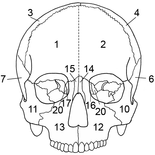
Skull, anterior view.
Zones
1. Right frontal, split sagittally through the metopic suture
2. Left frontal, split sagittally through the metopic suture
3. Right parietal
4. Left parietal
6. Left temporal, including the root of the zygomatic process
7. Right temporal, including the root of the zygomatic process
10. Left zygomatic bone
11. Right zygomatic bone
12. Left maxilla
13. Right maxilla
14. Left nasal bone
15. Right nasal bone
16. Left lacrimal bone
17. Right lacrimal bone
20. Ethmoid
22. Left inferior nasal concha (not depicted)
23. Right inferior nasal concha (not depicted)
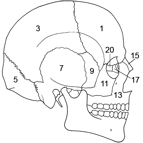
Skull, lateral right view.
Zones
1. Right frontal, split sagittally through the metopic suture
3. Right parietal
5. Occipital
7. Right temporal, including the root of the zygomatic process
9. Right sphenoid
11. Right zygomatic bone
13. Right maxilla
15. Right nasal bone
17. Right lacrimal bone
20. Ethmoid
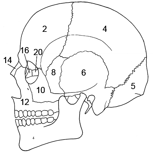
Skull, lateral left view.
Zones
2. Left frontal, split sagittally through the metopic suture
4. Left parietal
5. Occipital
6. Left temporal, including the root of the zygomatic process
8. Left sphenoid
10. Left zygomatic bone
12. Left maxilla
14. Left nasal bone
16. Left lacrimal bone
20. Ethmoid
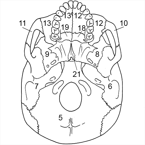
Skull, inferior view.
Zones
5. Occipital
6. Left temporal, including the root of the zygomatic process
7. Right temporal, including the root of the zygomatic process
8. Left sphenoid
9. Right sphenoid
10. Left zygomatic bone
11. Right zygomatic bone
12. Palatal process of the left maxilla
13. Palatal process of the right maxilla
18. Left palatine bone
19. Right palatine bone
21. Vomer
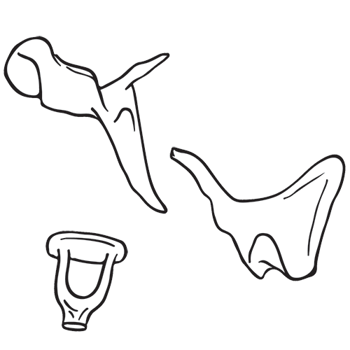
Ear ossicles. Top to bottom: malleus, incus, and stapes.
Zones
Ear ossicles
1. Present or absent
Mandible
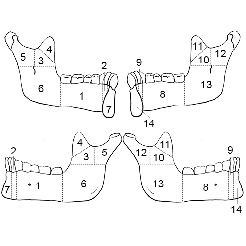
Mandible. Top left: medial/internal view of left; Top right: medial/internal view of right; Bottom left: lateral/external view of left; Bottom right: lateral/external view of right.
Zones
1. Portion of the left corpus, including alveoli for the premolars and molars as well as the premolars and molars themselves
2. Portion of the left corpus, including alveolus for the canine and the canine itself
3. Area of the left ascending ramus inferior to the coronoid process
4. Left coronoid process
5. Left mandibular condyle and the posterior portion of the ascending ramus
6. Left gonial angle, including the mandibular foramen and mylohyoid groove (internally) and the attachment of M. masseter (externally)
7. Anterior portion of the left corpus, including the alveoli of the incisors and the incisors themselves
8. Portion of the right corpus, including alveoli for the premolars and molars as well as the premolars and molars themselves
9. Portion of the right corpus, including alveolus for the canine and the canine itself
10. Area of the right ascending ramus inferior to the coronoid process
11. Right coronoid process
12. Right mandibular condyle and the posterior portion of the ascending ramus
13. Right gonial angle, including the mandibular foramen and mylohyoid groove (internally) and the attachment of M. masseter
externally)
14. Anterior portion of the right corpus, including the alveoli of the incisors and the incisors themselves
POSTCRANIAL REMAINS
Vertebrae and hyoid
Hyoid
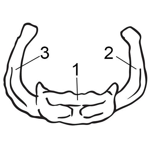
Hyoid. Anterior view.
Zones
1. Hyoid body
2. Left greater horn
3. Right greater horn
Cervical vertebrae
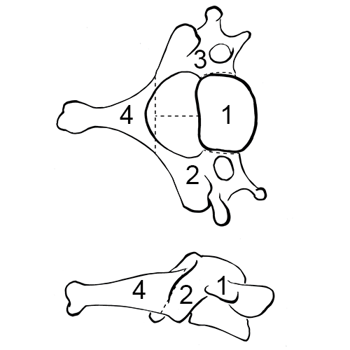
Cervical vertebra. Above: superior view; below: lateral view.
Zones
1. Body
2. Right transverse process, including the pedicle, pars interarticularis, and articular facets
3. Left transverse process, including the pedicle, pars interarticularis, and articular facets
4. Spinous process
Thoracic and lumbar vertebrae
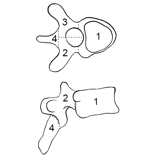
Thoracic vertebra (also applies to lumbar vertebrae). Above: superior view, below: lateral view.
Zones
1. Body
2. Right transverse process, including the pedicle, pars interarticularis, and articular facets
3. Left transverse process, including the pedicle, pars interarticularis, and articular facets
4. Spinous process
Sacrum
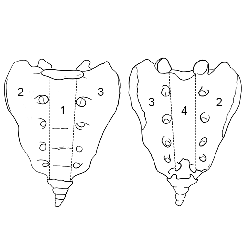
Sacrum. Left: anterior view; right: posterior view.
Zones
1. Body
2. Right transverse process, including the pedicle, pars interarticularis, and articular facets
3. Left transverse process, including the pedicle, pars interarticularis, and articular facets
4. Spinous process
Thorax and Shoulder
Rib 1
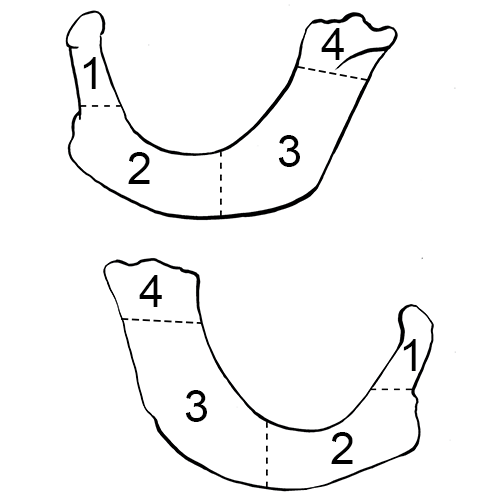
Left rib 1. Above: inferior view; below: superior view.
Zones
1. Head
2. Rib angle including tubercle
3. Corpus
4. Sternal end
Ribs 2-12
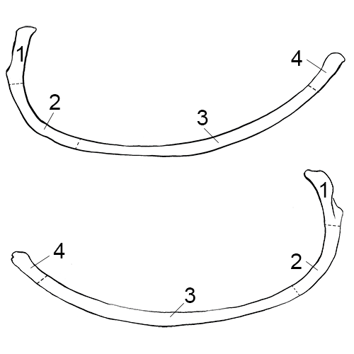
Left rib 7. Above: inferior view; below: superior view.
Zones
1. Head and tubercle
2. Rib angle including the articular and non-articular costal facets in ribs 1 through 10
3. Corpus
4. Sternal end
Sternum
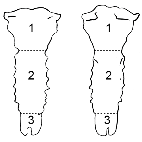
Sternum. Left: anterior view; right: posterior view.
Zones
1. Manubrium
2. Corpus sterni
3. Xiphoid process
Clavicle
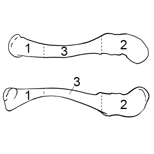
Left clavicle. Above: superior view; below: inferior view.
Zones
1. Sternal end, including the area of the attachment for the costo-clavicular ligament
2. Acromial end, including the conoid tubercle and trapezoid line
3. Diaphysis, including the groove that marks the attachment for M. subclavius
Scapula
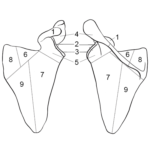
Left scapula. Left: anterior view; right: posterior view.
Zones
1. Coracoid process
2. Superior half of the glenoid cavity
3. Inferior half of the glenoid cavity
4. Acromial end and axillary/lateral third of the spine
5. Axillary/lateral third of the squamous portion and spine, including the neck and the area inferior to the coracoid process
6. Middle third of the supraspinous fossa and middle third of the scapular spine
7. Axillary/lateral half of the squamous portion inferior to the spine, including the infraspinous fossa
8. Vertebral third of the squamous portion and spine, including the attachment for M. rhomboideus major and suprasprinous fossa
9. Vertebral half of the squamous portion inferior to the spine, including the infraspinous fossa
Upper limb
Humerus
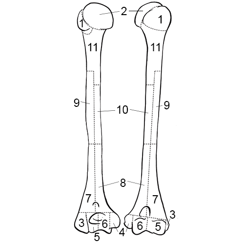
Left humerus. Left: posterior view; right: anterior view.
Zones
1. Greater and lesser tubercles
2. Caput
3. Lateral epicondyle
4. Medial epicondyle
5. Lateral articular process (capitulum) of the condyle
6. Medial articular process (trochlea) of the condyle
7. Distal lateral half of the diaphysis, including one-half of the olecranon fossa and the radial fossa
8. Distal medial half of the diaphysis, including one-half of the olecranon fossa and the coronoid fossa, including the nutrient foramen
9. Area surrounding the deltoid tuberosity
10. Area opposite zone 9 making up one-half of the diaphysis longitudinally in the sagittal plane and cutting the bone transversely from medial to lateral
11. Proximal portion of the diaphysis, including the surgical neck
Radius
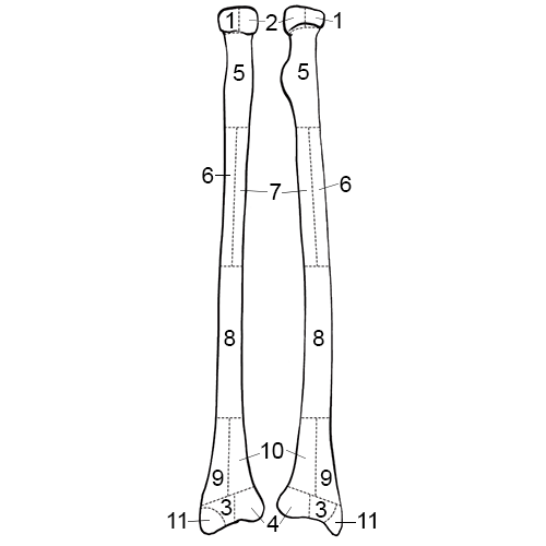
Left radius. Left: posterior view; right: anterior view.
Zones
1. Lateral half of the radial head
2. Medial half of the radial head
3. Lateral portion of the distal articulation
4. Medial portion of the distal articulation
5. Proximal portion of the diaphysis, including the radial tuberosity
6. Lateral half of the diaphysis to the mid-point of the diaphysis, including the attachment for M. pronator teres
7. Medial half of diaphysis to the mid-point of the diaphysis, opposite zone 6, including the nutrient foramen, which is located antero-medially
8. Superior half of the distal third of the radius
9. Lateral distal third of the diaphysis
10. Medial distal third of the diaphysis
11. Styloid process of the distal end
Ulna
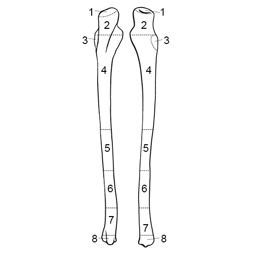
Left ulna. Left: posterior view; right: anterior view.
Zones
1. Olecranon process
2. Area of the trochlear or semi-lunar notch, including the coronoid process
3. Radial notch
4. Proximal half of the diaphysis distal to zone 3, including the nutrient foramen, which is located antero-medially
5. Middle portion of the diaphysis
6. Superior one-half of the distal third of the diaphysis
7. Distal half of the distal third of the diaphysis, including the attachment of M. pronator quadratus
8. Styloid process and head, including the posterior groove for M. extensor carpi ulnaris
Pelvis and Lower Limb
Os coxa
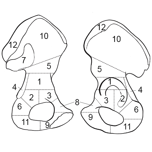
Left os coxa. Left: medial/internal view; right: lateral/external view.
Zones
1. Superior portion of the acetabulum and adjoining areas anteriorly and posteriorly
2. Posterior half of the inferior portion of the acetabulum and adjoining areas
3. Anterior half of the inferior portion of the acetabulum and adjoining areas
4. Superior portion of the ischium, including the ischial spine
5. Inferior portion of the ilium, including the greater sciatic notch
6. Superior portion of the ischial tuberosity
7. Auricular surface of the ilium
8. Superior portion of the pubis possessing the pectineal line and pubic tubercle
9. Inferior portion of the pubis, including the pubic symphysis
10. Greater part of the ilium, marked in an antero-posterior diretion by a line running from just inferior to the anterior superior iliac spine to the posterior inferior iliac spine, but not including the iliac crest (superiorly)
11. Inferior portion of the ischial tuberosity
12. Iliac crest
Femur
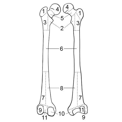
Left femur. Left: posterior view; right: anterior view.
Zones
1. Greater trochanter
2. Area around the lesser trochanter and the lesser trochanter
3. Area of the cranial attachment of M. gluteus maximus
4. Caput
5. Neck of the element and area along the inter-trochanteric line (anteriorly) and intertrochanteric crest (posteriorly)
6. Middle portion of the diaphysis to the point where the linea aspera bifurcates into the supra-condylar lines, including the nutrient foramen, which is located posteriorly
7. Lateral half of the distal third of the diaphysis split longitudinally in the sagittal plane, including one-half of the popliteal space (posteriorly)
8. Medial half of the distal third of the diaphysis split longitudinally in the sagittal plane, including one-half of the popliteal space (posteriorly)
9. Lateral condyle and epicondyle
10. Medial condyle and epicondyle
11. Intercondylar space and distal articulation anteriorly
Patella
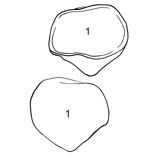
Left patella. Above: posterior view; below: anterior view.
Tibia
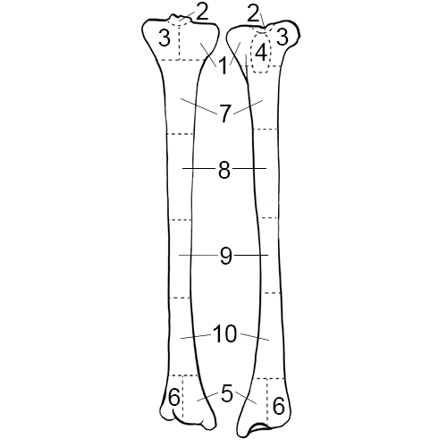
Left tibia. Left: posterior view; right: anterior view.
Zones
1. Medial proximal condyle
2. Intercondylar fossa between the tibial spines, including the area of attachment of the posterior cruciate ligament
3. Lateral proximal condyle
4. Area of the tibial tuberosity
5. Area of the medial malleolus
6. Area of the lateral malleolus
7. Proximal quarter of the diaphysis, including the nutrient foramen, which is located posteriorly
8. Second quarter of the diaphysis
9. Third quarter of the diaphysis
10. Distal quarter of the diaphysis
Fibula
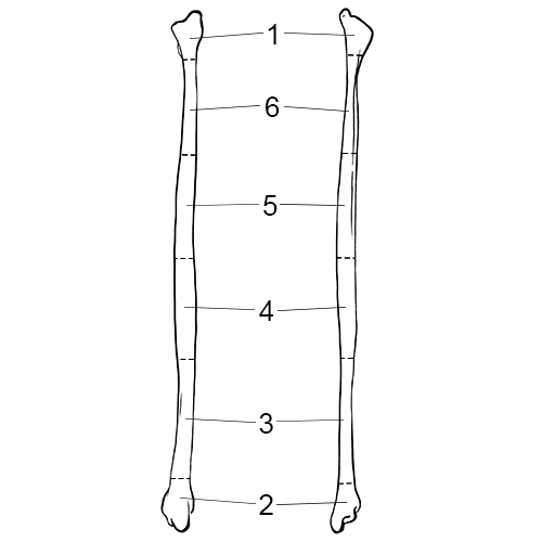
Left fibula. Left: anterior view; right: posterior view.
Zones
1. Proximal end, essentially the juvenile epiphysis, including the styloid process
2. Distal end, essentially the juvenile epiphysis
3. Most distal quarter of the diaphysis, including the attachment for the inferior portion of the interosseous ligament (a triangular rugose region with its apex directed anteriorly)
4. Middle quarter of the diaphysis, including the nutrient foramen, which is located posteriorly
5. Second quarter of the diaphysis
6. Most proximal quarter of the diaphysis, distal to the juvenile epiphysis
Hands and Feet
Hand
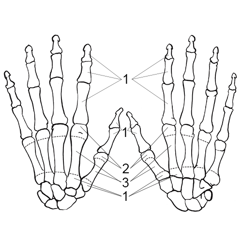
Left hand and wrist. Left: dorsal view; right: palmar view.
Zones
Carpals and phalanges
1. Present or absent
Metacarpals
1. Proximal articulation
2. Distal articular condyle
3. Diaphysis
Foot
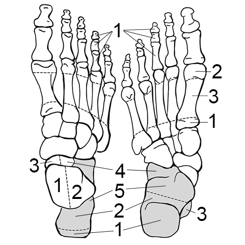
Right foot and ankle. Left: dorsal view; right: plantar view.
Zones
Calcaneus
1. Tuber calcis
2. Distal portion of the body
3. Sustentaculum tali
4. Proximal articulation
5. Proximal portion of the body inferior to the articulations
Talus
1. Medial half of the trochlea
2. Lateral half of the trochlea
3. Medial half of the proximal portion, splitting the head sagittally
4. Lateral half of the proximal portion, splitting the head sagittally
Remaining tarsals and phalanges
1. Present or absent
Metatarsals
1. Proximal articulation
2. Distal artiuclar condyle
3. Diaphysis
-
Knüsel, C.J. and A.K. Outram (2004) Fragmentation: The zonation method applied to fragmented human remains from archaeological and forensic contexts. Environmental Archaeology 9:85-98.Material 2.0.* University of Tennessee and Lincoln Memorial University ↩
-
Langley, N.R., L.M. Jantz, S.D Ousley, R.L. Jantz, and G. Milner (2016) Data Collection Procedures for Forensic Skeletal Material 2.0. University of Tennessee and Lincoln Memorial University ↩
Field attributes
Field Attributes
New Skeletal Element Page
Accession (required field)
- Tracking identifier, such as a laboratory or project name and/or number
- Alphanumeric
- Minimum of three characters
- Example: 2018-001 or ABC 2018-001
Provenance 1
- Secondary tracking identifier, such as information related to grave, casket, or recovery provenience
- Alphanumeric
- Example: A-01
Provenance 2
- Additional tracking identifier, such as additional information related to grave, casket, recovery provenience, or bag number
- Number(s) and/or letter(s)
- Example: A2
Designator (required field)
- Unique number for the element
- Alphanumeric
- No special characters or symbols
- Example: 101
Bone (required field)
- Choose element from drop-down list
- Options exist for unidentifiable elements (Ex: Unidentified cervical vertebra, unidentified long bone)
Side (required field)
- Left – element is from the left side of the body
- Right – element is from the right side of the body
- Middle – element is from the middle of the body (Ex: cranium, thoracic vertebra 1)
- Unsided – any element that side cannot be determined
Completeness (required field)
- Complete – a complete element is present, fragmentary or whole → If complete is chosen, all zones will be automatically populated
- Incomplete – any element that is not complete
Click “save” to continue analysis. All fields can be edited/updated after the element has been saved, until “Inventoried” is checked, then changes cannot be made without approval by the project lead/manager/creator/etc.
View Skeletal Element Page
Same fields as “New Skeletal Element” with the addition of:
To enter or edit data, you must go to Actions → Edit
CT Scanned
- Check this box if element has been CT scanned
X-ray Scanned
- Check this box if element has been x-rayed
Clavicle Triage
- Check this box if element has been triaged for chest radiograph comparison
Measured
- Box will automatically be checked when any measurements are saved under the Measurements analysis
DNA Sample
- Box will automatically be checked when any measurements are saved under the DNA Profile analysis
Inventory Completed
- Check this box if inventory is complete and is ready for review
- Information cannot be changed once this box is checked. Changes cannot be made without approval by the project lead/manager/creator/etc.
Reviewed
- Check this box if review is complete
Individual Number
- Unique identifier given when element is being associated as an individual, i.e., multiple elements representing a single individual are given one number
- Example: 2018-IND-1 or IND 2018-001
Click Details to add Analyses
Analysis
Biological Profile
Age
- Choose the applicable method; this list is based on methods applicable to the element. Click Create.
- Fill in appropriate age scores/descriptions. Click Save.
- Information can be edited after save, but cannot be deleted.
Sex
- Choose the applicable method; this list is based on methods applicable to the element. Click Create.
- Fill in appropriate scores/descriptions. Click Save.
- Information can be edited after save, but cannot be deleted.
Stature
- No methods available.
Ancestry
- Choose the applicable method; this list is based on methods applicable to the element. Click Create.
- Fill in appropriate scores/descriptions. Click Save.
- Information can be edited after save, but cannot be deleted.
DNA Profile
Lab
- Choose the laboratory that is conducting the DNA analysis
External Case #
- The DNA testing laboratory’s case number
- Alphanumeric
DNA Sample Number
- The sample number for the DNA sample
- Alphanumeric
Mito Sequence Number
- mitochondrial DNA sequence number
- Numeric
Mito Sequence Subgroup
- mitochondrial DNA sequence number
- Alphanumeric
Mito Sequence Similar
- If there is a similar mitochondrial DNA sequence number, list it here
- Alphanumeric
Mito Match Count
- Number of individuals matching the mitochondrial DNA sequence
- Numeric
Mito Total Count
- Total number of individuals in the reference/comparison group
- Numeric
Once saved, additional “analysis tests” can be added
Taphonomy
Chose appropriate taphonomic description for the following categories: * General color * Adherent materials * Biological * Burned * Physical * Staining * Human modification
Numerous descriptors can be chosen * Can be deleted after clicking “save”
Zonal Classification
- Check the box for the corresponding zone that is present.
- As a general rule, check a zone present if ≥50% of the zone is present.
Measurements
- Must be numeric, not more than two decimal places
- Ex: 241, 13.5, 14.56
- Must click “save”
- Can be deleted after clicking “save”
Associations
Articulations
• Select articulating element(s)
Pair Matching
• Select pair matching element(s)
Refits
• Select refitting element(s)
Pathology
Trauma
By zone description of type of trauma, with free text space for additional information.
Options include the following, as a general category or a specific type of trauma:
- Antemortem
- Perimortem
Pathology
By zone description of type of pathology, with free text space for additional information.
Options include the following, as a general category or a specific type of pathology:
- Density
- Morphology
- Proliferative
- Lytic
- Deformative
Anomaly
Choose any anomaly description available
Analytics & Visualizations
What is CoRA Analytics?
The CoRA Analytics engine is part of the CoRA Ecosystem that can be thought of as an extension and a framework to perform analytics on forensic anthropology datasets. It is also designed to act as a broker facilitating exchange of data from various systems such as the native CoRA projects data, CMS/StarLIMS data in the appropriate format and sending the various datasets to the appropriate analytics apps. These analytics apps can be independent self contained applications build by individual researchers and are independent of the CoRA Ecosystem developed and managed by the researcher/author. These apps must follow and comply with established architecture guidelines to work with the base CoRA Analytics engine and established data quality parameters and established APIs.
The diagram below details the logical diagram for the CoRA Ecosystem Analytics Architecture.
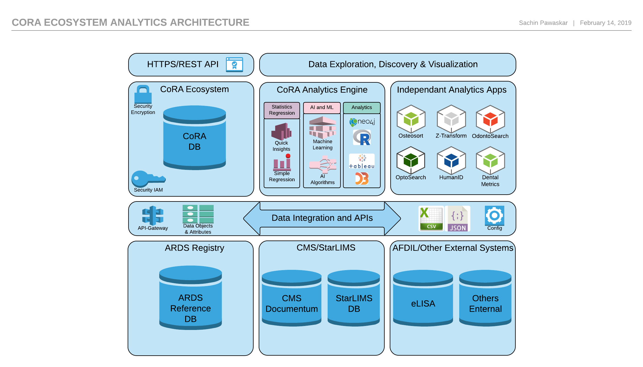
Dashboard Visualizations
Warning
The following section on this page is work in progress.
Built-in Analytics
The CoRA analytics engine provides some built-in analytics out of the box such as simple regression analysis for the datasets that are most commonly used in forensic anthropology. Other more advanced analytics will be provided via independent analytics application that can be developed by any researcher and plug-in into the CoRA Ecosystem.
Knowledge Graphs
The CoRA analytics engine provides the ability to leverage advanced analytics using project specific knowledge graphs. The CoRA knowledge graphs leverages the Neo4J Graph database to allow forensic anthropologists and scientists to better understand & analyze their project specimens and its related data to help in the missing persons identification process. It allows forensic scientists to find relationships between specimens using related data such as DNA, pair matching, articulations, taphonomy, anomaly, trauma, pathology, among others.
So What is a Knowledge Graph?
A knowledge graph is a design pattern for storing, organizing, and accessing interrelated data entities, including their semantic relationships. With knowledge graphs, you can better understand your data and build more intelligent applications. A knowledge graph contains three essential elements:
- Entities, which represent the data of the organization or domain area.
- Relationships, which show how the data entities interact with or relate to each other. Relationships provide context for the data.
- An organizing principle that captures meta-information about core concepts relevant to the business.
Here is the process guide that project leads and their teams can use to get access to their projects knowledge graph DBMS.
Independent Analytics Applications
Following are some of the independent analytics applications that are either being developed or have already been developed that work with the CoRA Ecosystem.
Independent Analytics Applications
The following section on this page is work in progress.
Osteometric Sorting
Blurb by author here - Jeffery Lynch
Z-Transform
Blurb by author - Julia Sommer
Odontosearch
Blurb by author here - Author Name
Optosearch
Blurb by author here - Author Name
HumanID
Blurb by author here - Author Name
Dental Metrics
Blurb by author here - Author Name
Contribution Guidelines for CoRA Analytics
Built-in analytics
Built-in Analytics
The CoRA analytics engine provides some built-in analytics out of the box such as simple regression analysis for the datasets that are most commonly used in forensic anthropology. Along with these CoRA provides some visualizations that you might find very useful in narrowing down the search space as you work on the segregation process.
Please note that built-in analytics and visualization are worked on at a regular basis to fine tune their performance. Please consider these to be in experimentation phase until final release. You are encouraged to use the built-in analytics as is.
Info
We would appreciate your use of these analytics and visualizations and your feedback on making them better and more useful to you. Thank you.
Bipartite Graph
Warning
This page is work in progress.
Bipartite Graph
A Bipartite Graph allows you to visualize the bipartite data effectively. Here CoRA use it to demonstrate the matching specimens and its relationships in the form of a bipartite graph.
The following table shows the required and optional fields to generate a bipartite graph.
| Attributes | Required/Optional |
|---|---|
| Relations | Required |
| Bones | Required |
| Side | Required |
| Specimen | Required |
Steps to generate a Bipartite Graph.
Step 1: Select a relation
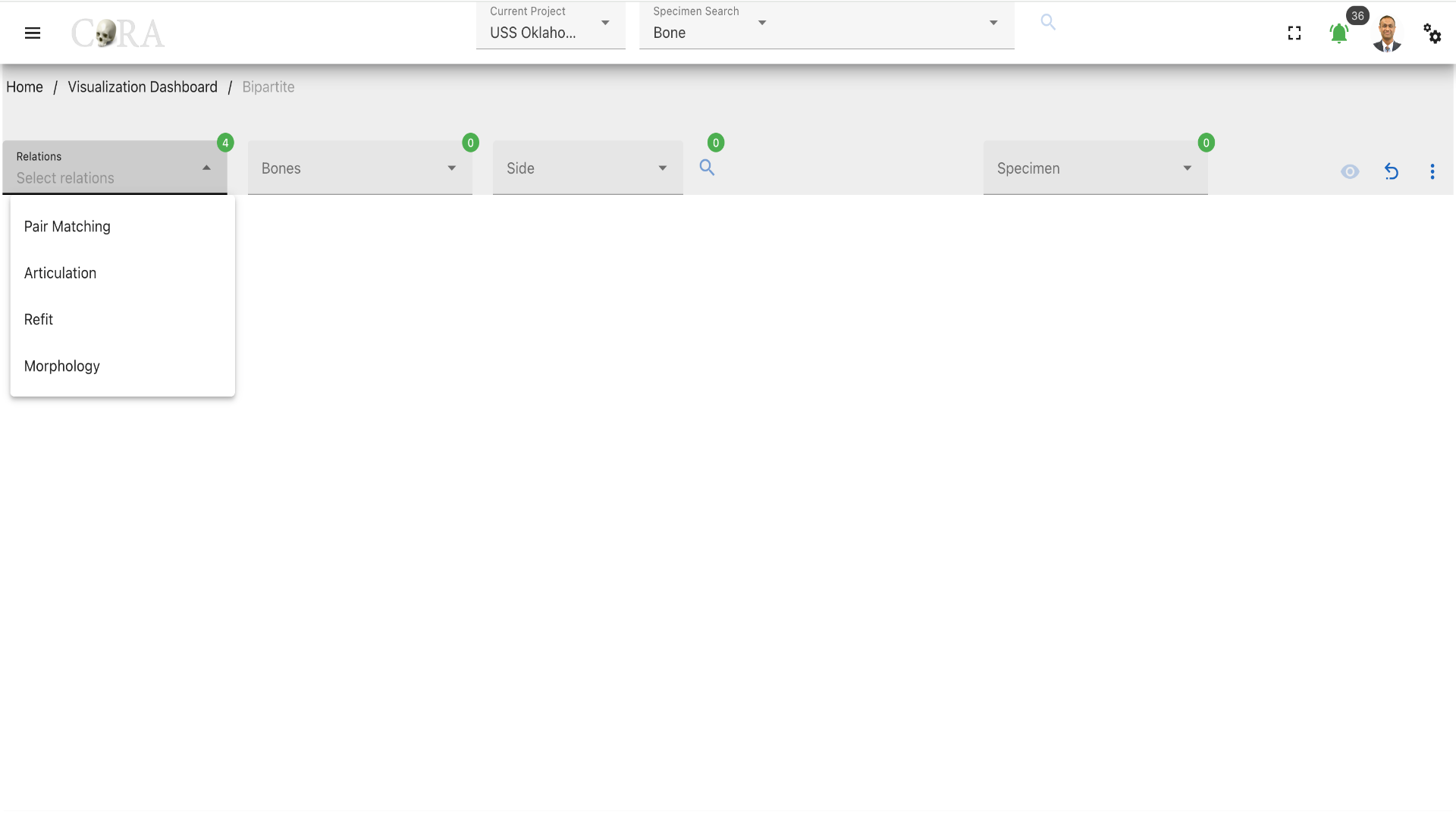
Select one from the four (4) association relations based on the requirement. The four (4) association relations available are:
- Pair Matching
- Articulation
- Refits
- Morphology
Step 2: Select a bone
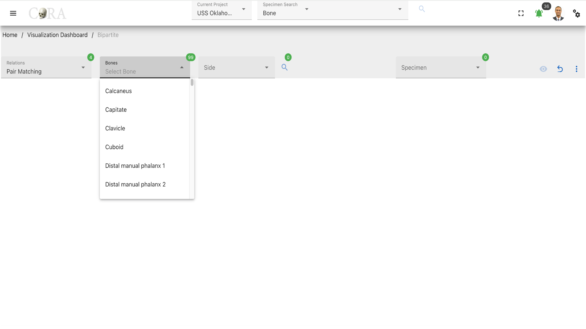
Select the bone type of the specimen from the available list of the bones required for the bipartite graph generation.
Step 3: Select a side
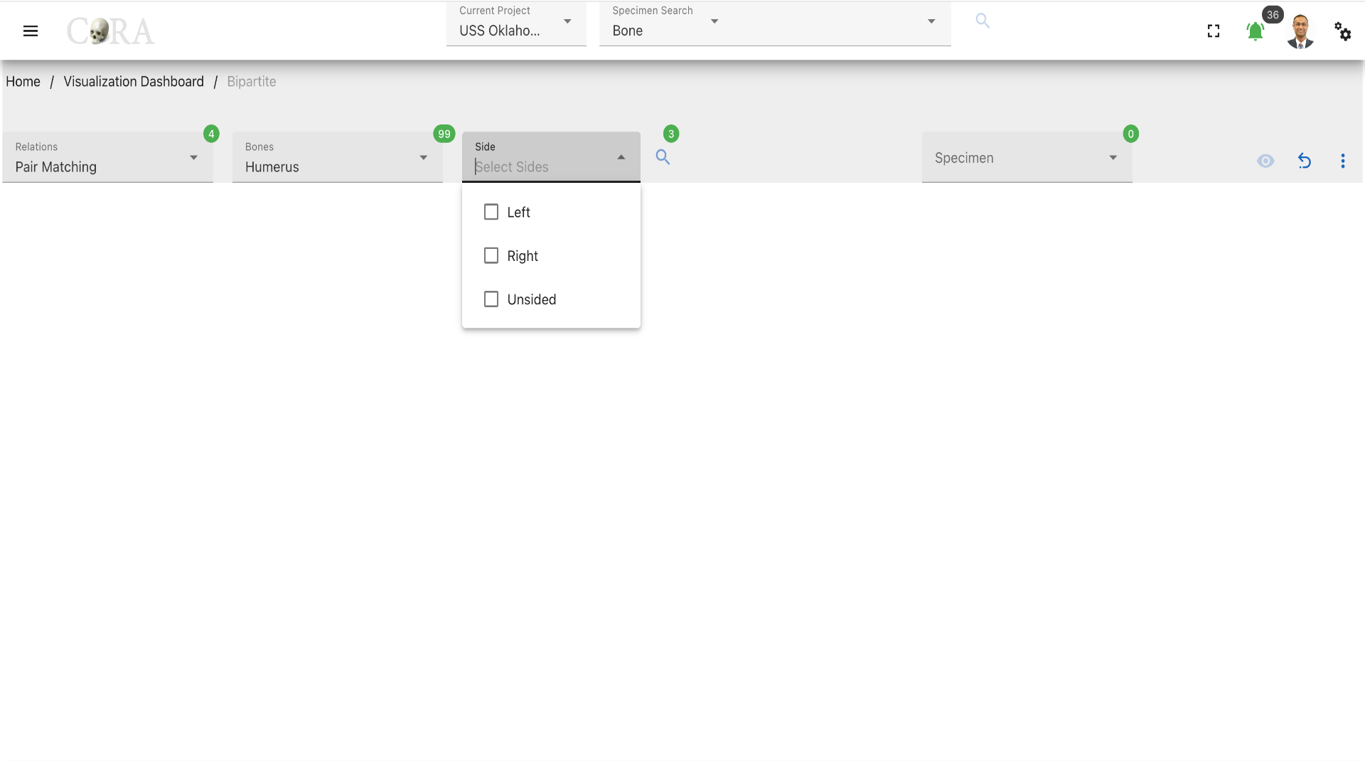 Select the bone side from the available dropdown list. After selecting the side click on the 'search' icon to generate the list of specimens based on the options selected previously. The following are the list of sides available:
- Left
- Right
- Unsided
Step 4: Select a Specimen
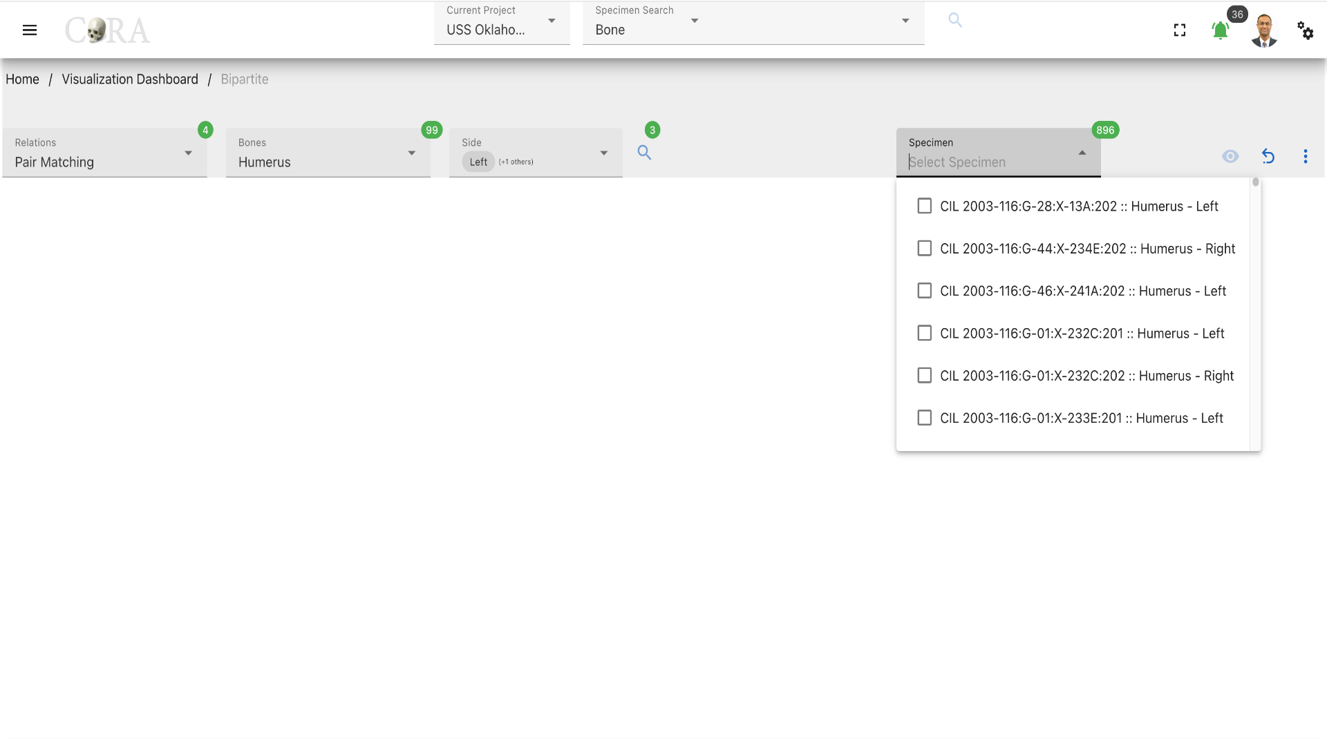 Select one or more specimen based on the analytics requirement and click on the 'eye' icon to generate the visualization. Now click on any of the colors on the generation to view the relationship in the specimen selected.
More Options/Filters
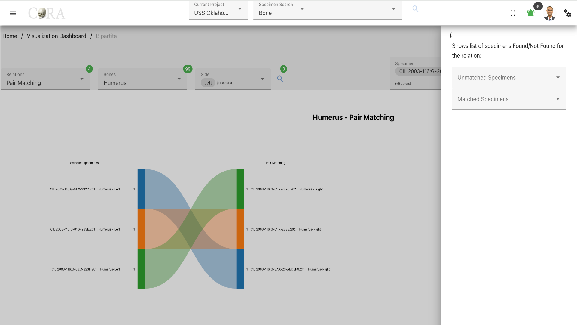 Click on the kebab menu icon to view more options of the list of specimens Found/Not Found for the relation and interact with the visualization.
Collapsible Tree
Warning
This page is work in progress.
Collapsible Tree
A Collapsible tree can present hierarchical data effectively. Here CoRA uses it to demonstrate specimens and its relationships in the form of a collapsible tree.
The following table shows the required and optional fields to generate a collapsible tree.
| Attributes | Required/Optional |
|---|---|
| Type | Required |
| Individual Number | Required |
| Accession Number | Required |
| Provenance 1 | Optional |
| Bone | Required |
| Specimen | Required |
Select a type
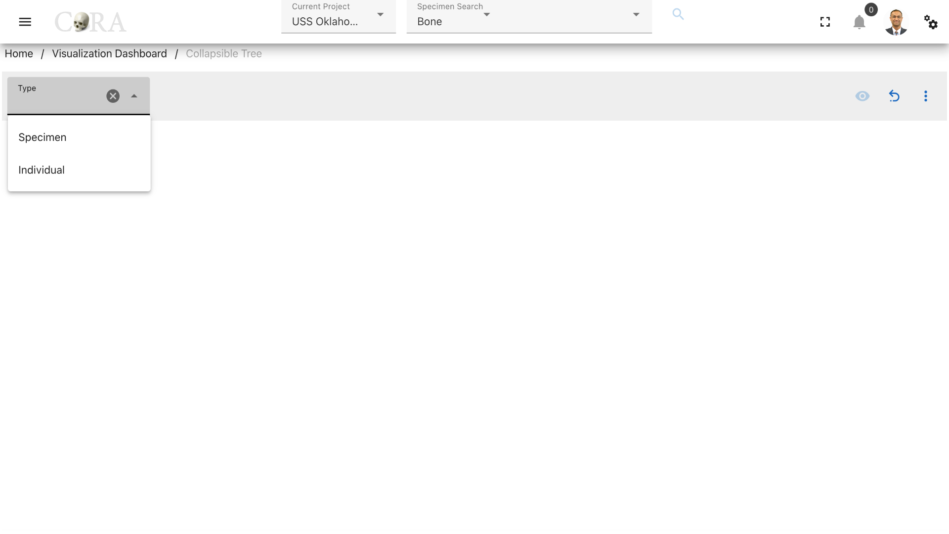
Select a type (specimen or individual) based on the analytics requirement. Select 'Specimen' based on a bone if a specimen is needed to be analyzed. Select 'Individual' if you want to analyze all the specimens that belong to an individual number.
Steps to generate a collapsible tree for 'Type: Specimen'
Step-1: Select accession number
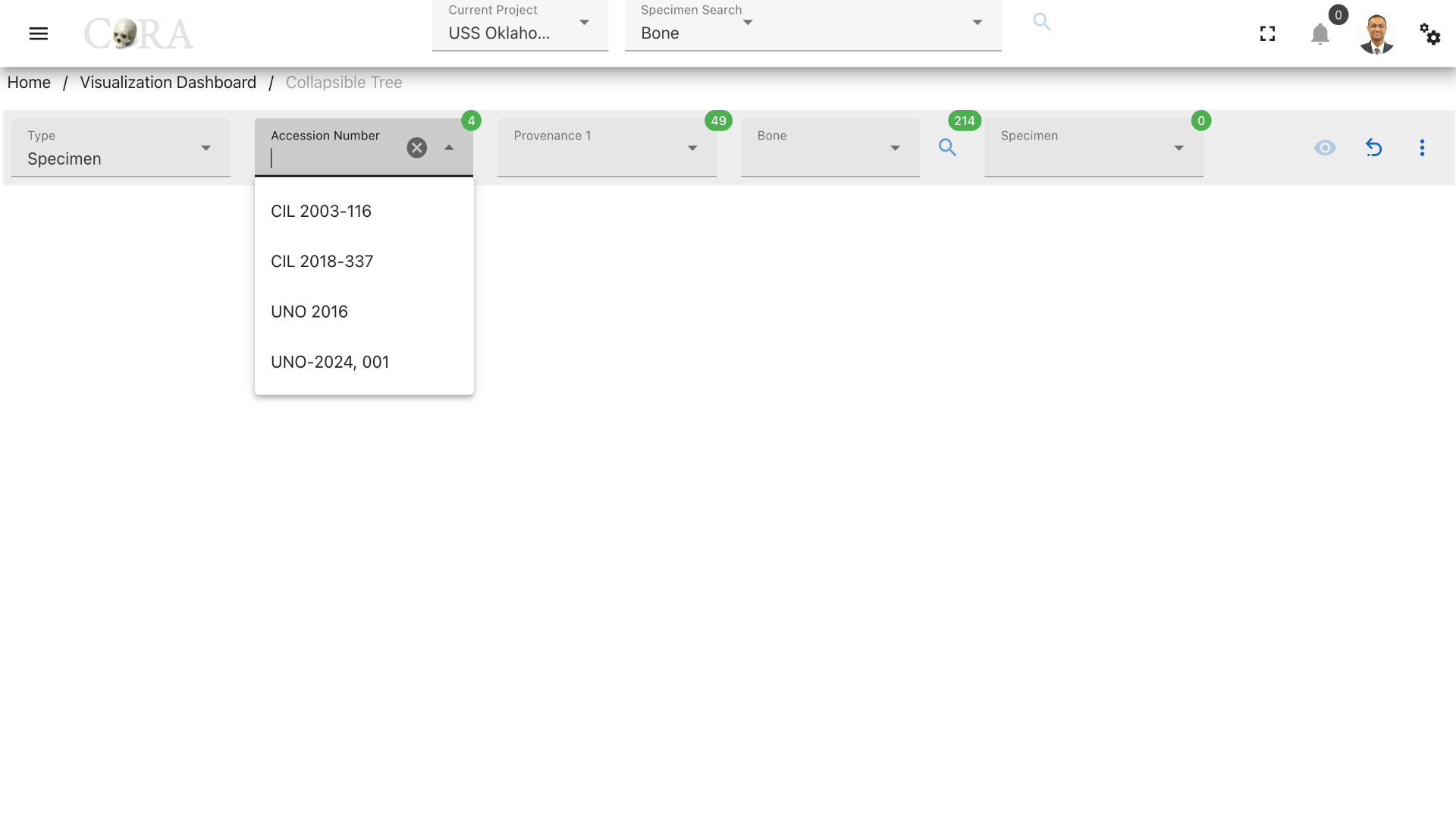
Select an accession number to which the required specimen belongs to.
Step-2: Select provenance1
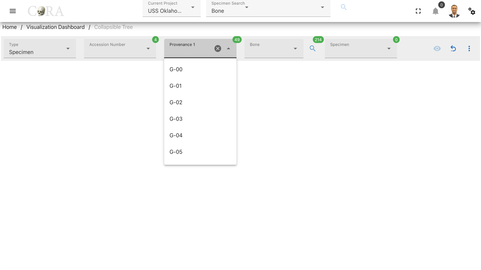
Select the provenance1 to which the required specimen belongs to. Note that choosing provenance1 is optional to generate the collapsible tree.
Step-3: Select bone
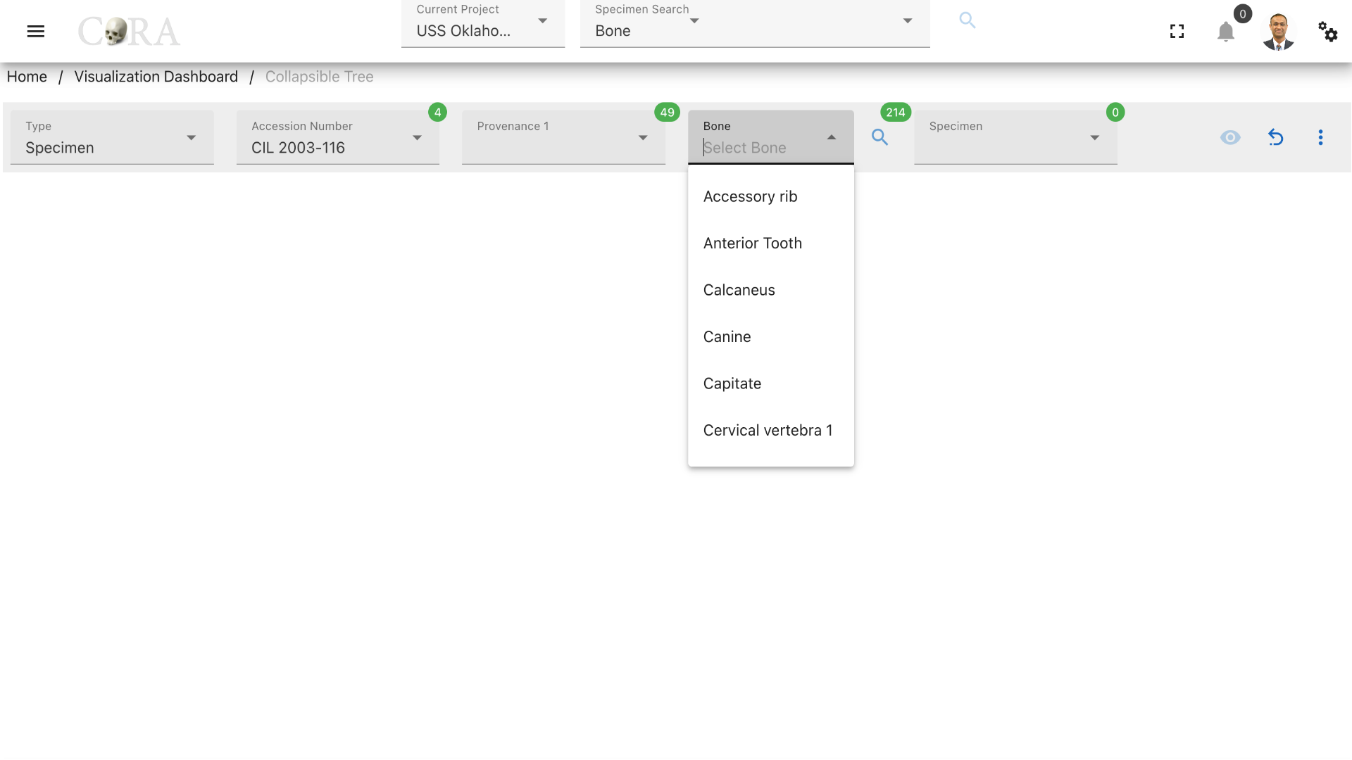
Select the bone type of the specimen from the available list of the bones. After selecting the bone type click on the 'search' icon to generate the list of specimens based on the options selected previously.
Step-4: Select specimen(s)
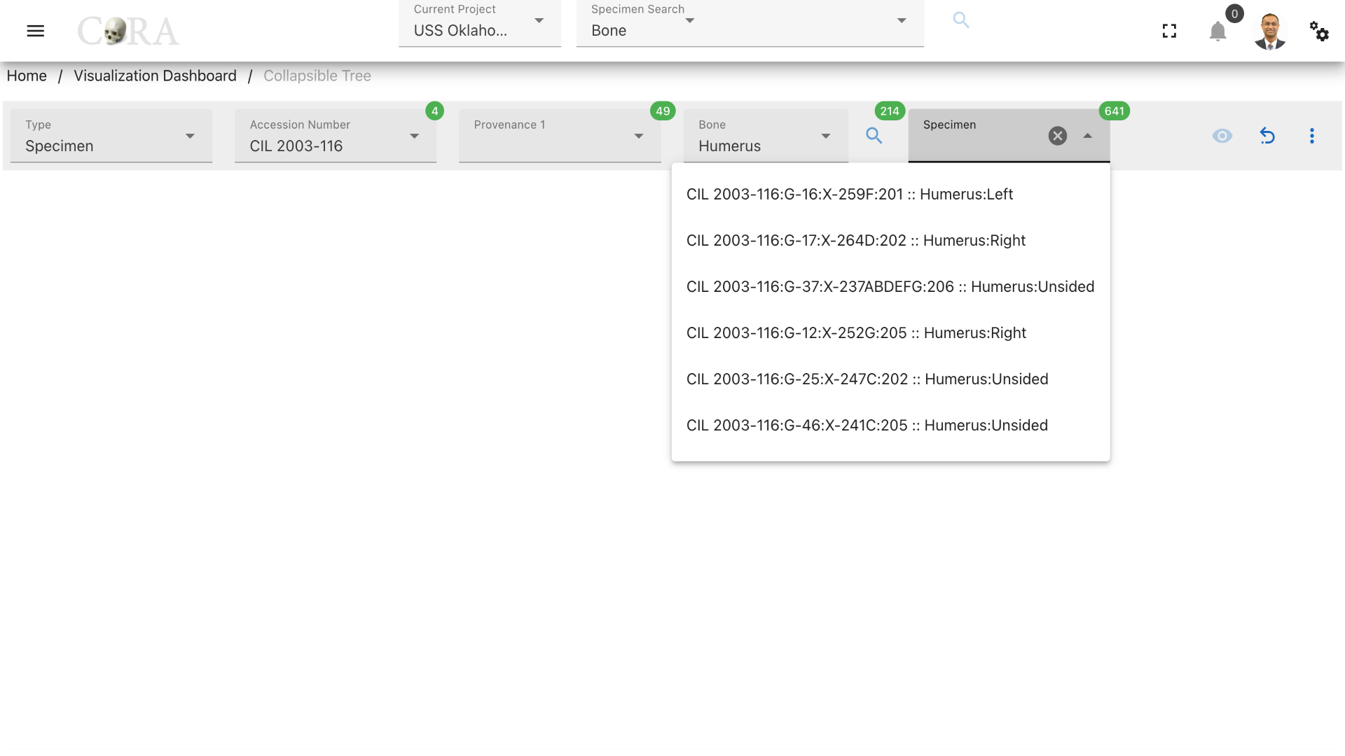
Choose the required specimens for which the collapsible tree is needed to be generated.
Step-5: Generate visualization
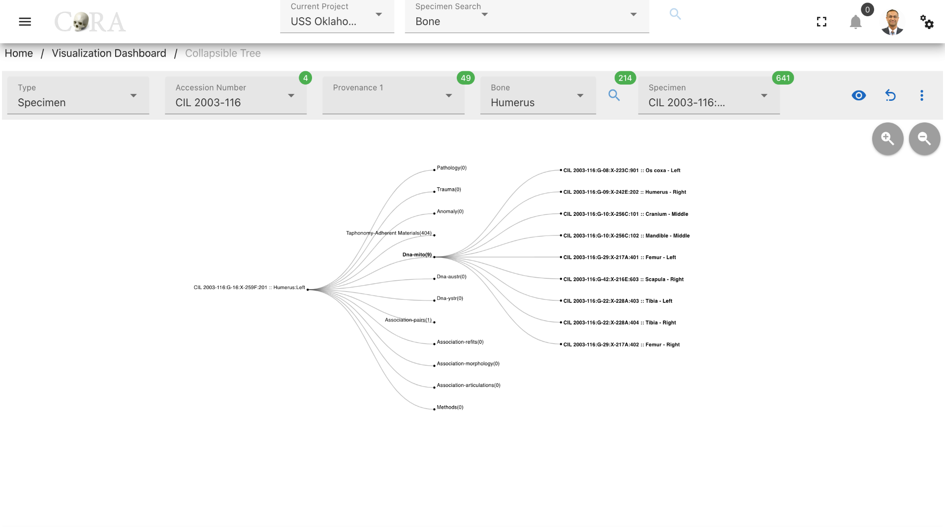
The collapsible tree can be generated by clicking on the 'eye' icon for the selected specimen. The collapsible tree can be further expanded by clicking on a specific relationship node which gives list of all related specimens and clicking on these specimens expands the tree even more by generating the relations of it again and the tree continues to grow.
Steps to generate a collapsible tree for 'Type: Individual'
Step-1: Select an individual number
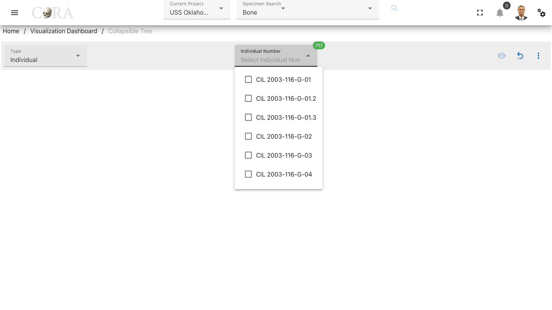
Select an individual number that you want to explore.
Step-2: Generate the collapsible tree
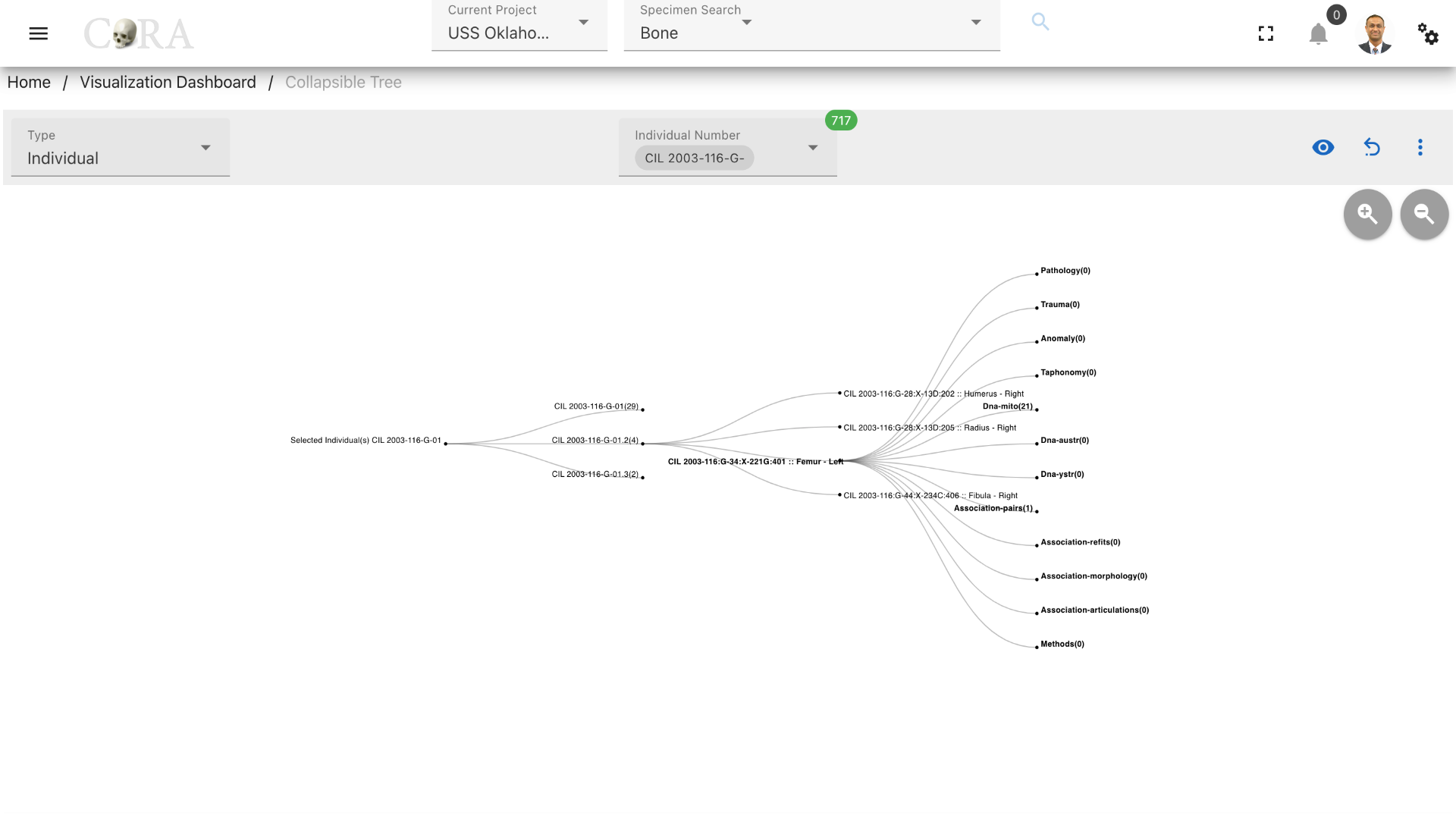
Click on the 'eye' icon to generate the collapsible tree. Now click on the necessary accession numbers and provenances to generate the list of specimens in the tree and further click on them similar to the specimens type tree to view the relations.
More Options/Filters:
Click on the kebab menu icon to view more options like removing relations with zero specimens, remove non-required relations and Provenance 2.
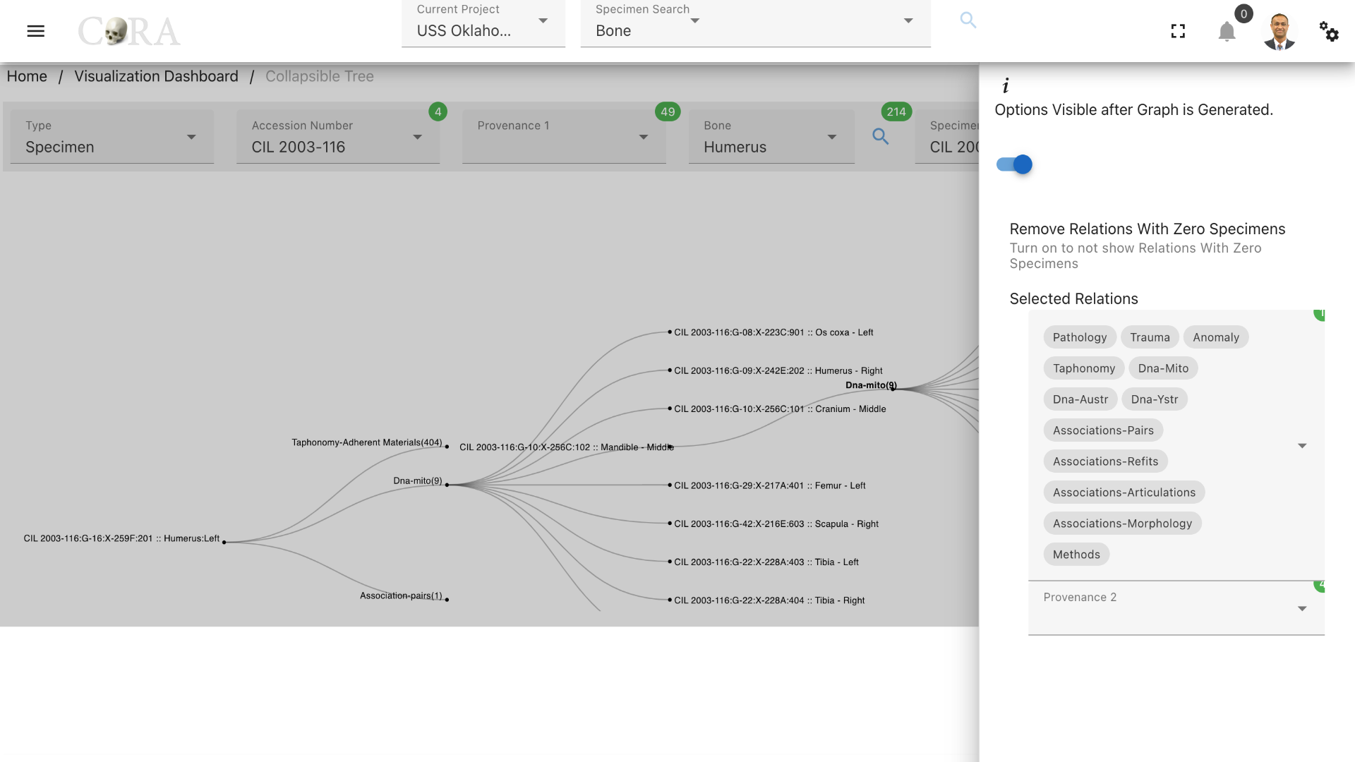
Use the toggle switch to remove relations with zero specimens and simplify the graph. Relations can also be removed individually under 'Selected Relations' based on the requirement. Provenance 2 can be used to further filter the specimens.
Available Specimen relationships
There are 12 possible relationships to explore
- pathology
- trauma
- taphonomy
- anomaly
- dnas-mito
- dnas-austr
- dnas-ystr
- methods
- associations-pairs
- associations-refits
- associations-articulation
- associations-morphology
DNA Visualization - MitoPolymorphisms
Note
This page describes how to visualize mitochondrial DNA polymorphisms and the modified reference sequence using the CoRA Visualization Dashboard.
Accessing DNA Visualization
Navigate to the DNA section via:
Left Sidebar Menu → Visualizations → DNA - Mitochondrial
This section allows for the visualization of mitochondrial DNA data associated with specific specimens.
Step 1: Select Filters
Use the filter dropdowns at the top of the page to refine your selection:
- Bones: e.g., Humerus
- Side: Left or Right
- Specimen
- DNA Sample Number
These selections drive which mutations and sequences are visualized on the chart and panel.
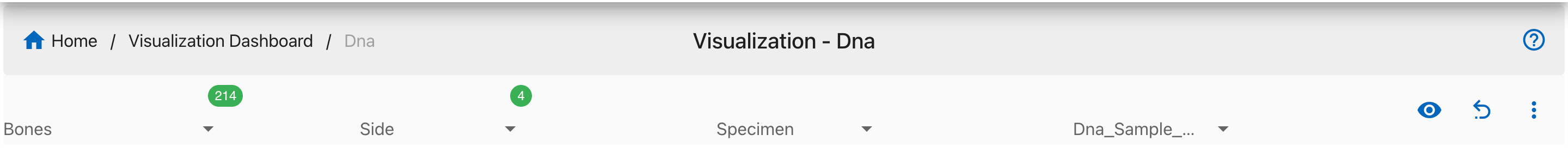
Step 2: Select a Bone and a Side
After selecting a Bone and a Side, Specimens and Dna_Sample_Number eye-button will be available. There are two ways we can create the visualizations mentioned below: 1. A - Select a Specimen then Dna_Sample_Number will be populated
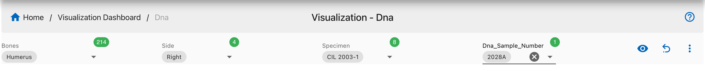
B - now when we click on eye button which will enable us to get the visualizations and its mutations.
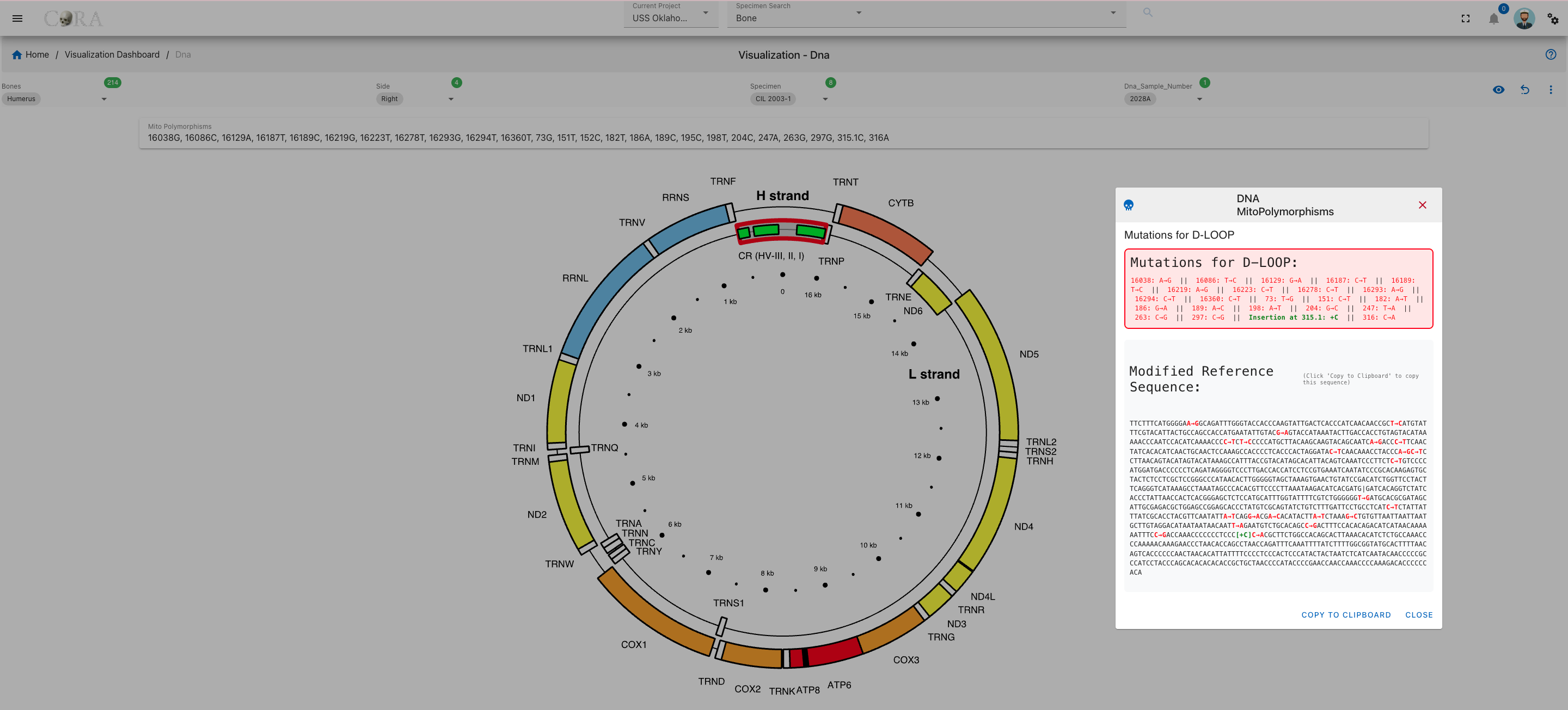
- After selecting Bone and side we can directly select the Dna_Sample_Number.

We can see the visualization
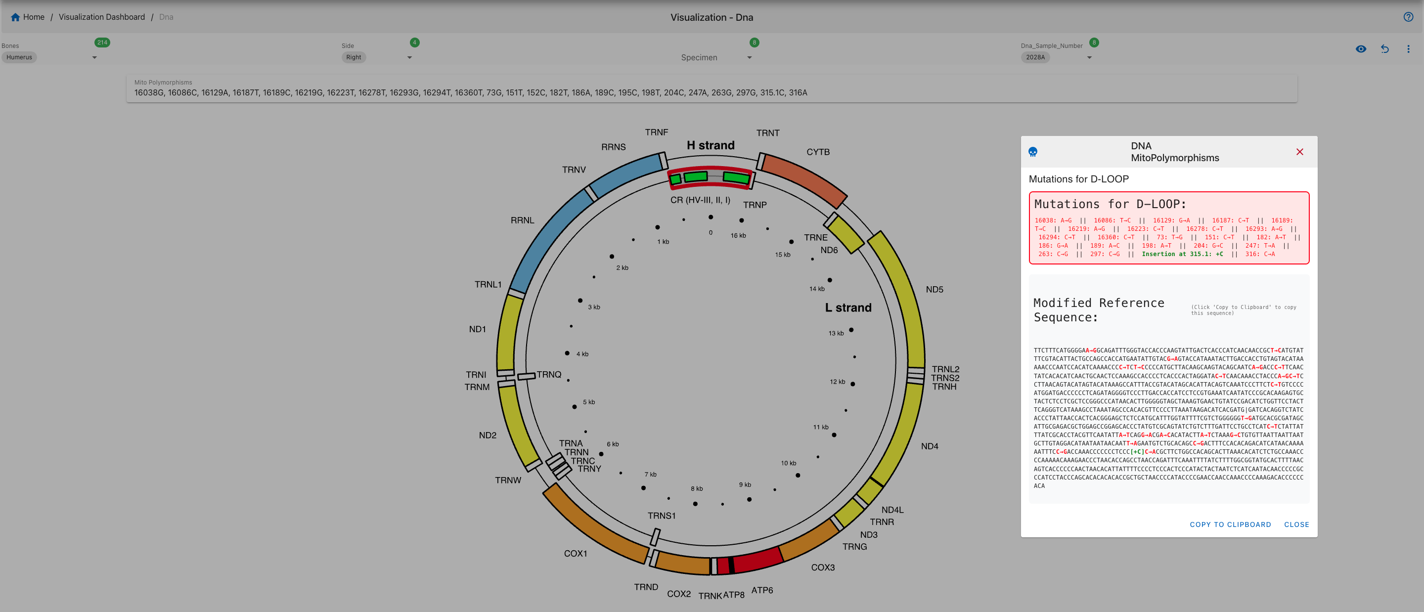
Step 3: View MitoPolymorphisms
Once a valid sample is selected, polymorphism data will be displayed in a circular mitochondrial genome viewer. respective region mutations will be highlighted.
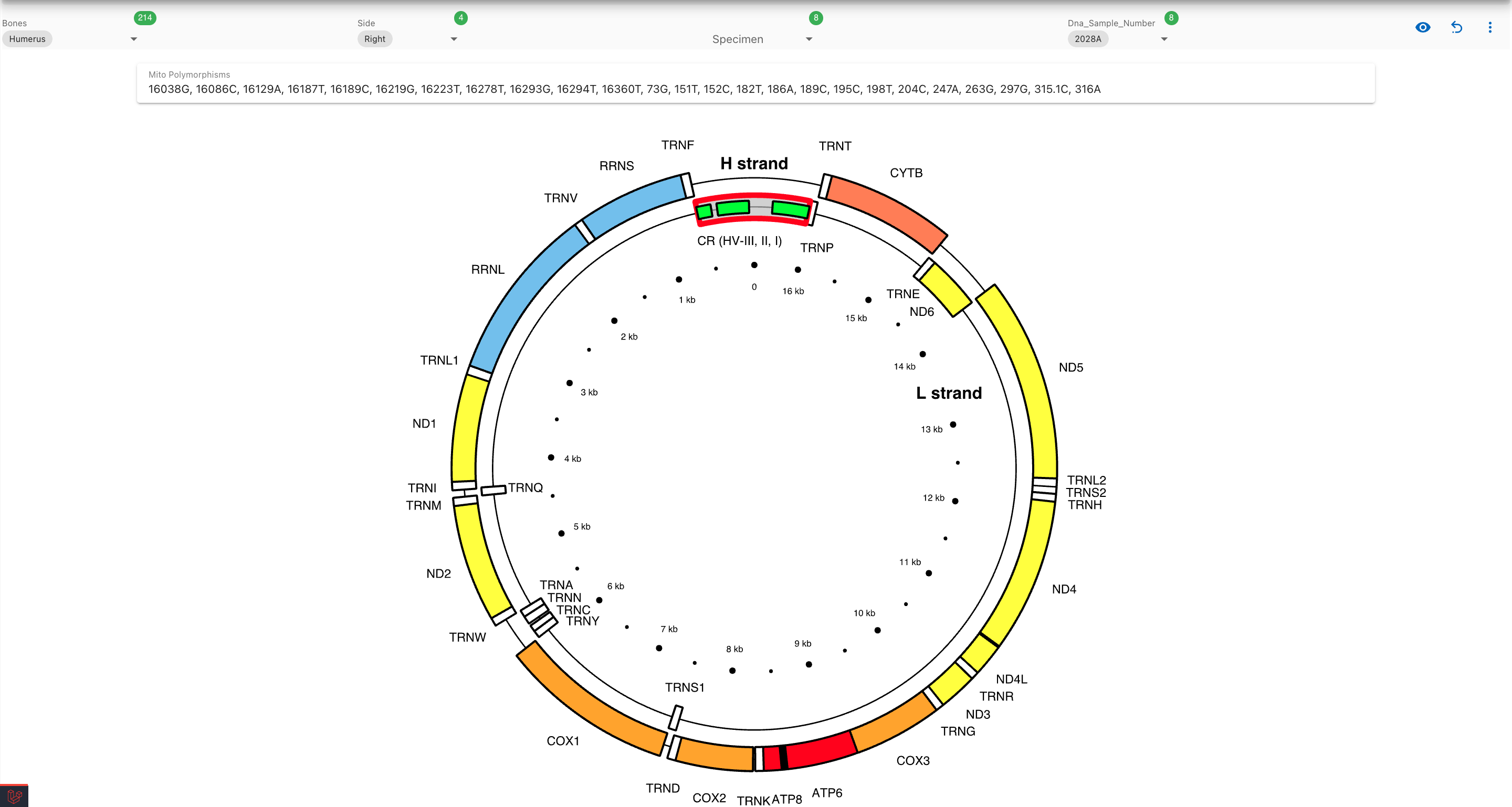
When we click on the highlighted region a mutation list is shown in a dialog box:
Hierarchical Clustering
Warning
This page is work in progress.
Hierarchical Clustering
Hierarchical clustering is a data analysis method that builds a hierarchy of clusters by either successively aggregating individual data points into clusters (agglomerate approach) or dividing a large cluster into smaller ones (divisive approach), based on their similarity.
In hierarchical clustering, the data is not partitioned into a particular cluster in a single step. Instead, clusters are formed sequentially, with each step involving the merging of the two nearest clusters at a lower level into a higher-level cluster. This process continues recursively until all data points are clustered into a single group or until the desired cluster structure is achieved.
The following table shows the required and optional fields to generate hierarchical clustering visualization
| Attributes | Required/Optional |
|---|---|
| Visualization Type | Required |
| Relationship | Required |
Steps to generate Hierarchical clustering graphs
Step-1: Select Visualization type
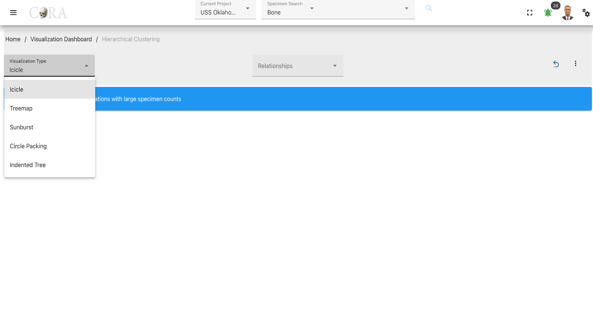
Select a type of visualization for the hierarchical clustering. The available visualization types are shown in the below table.
| Visualization Types |
|---|
| Icicle |
| Treemap |
| Sunburst |
| Circle Packing |
| Indented Tree |
Step-2: Select a relationship
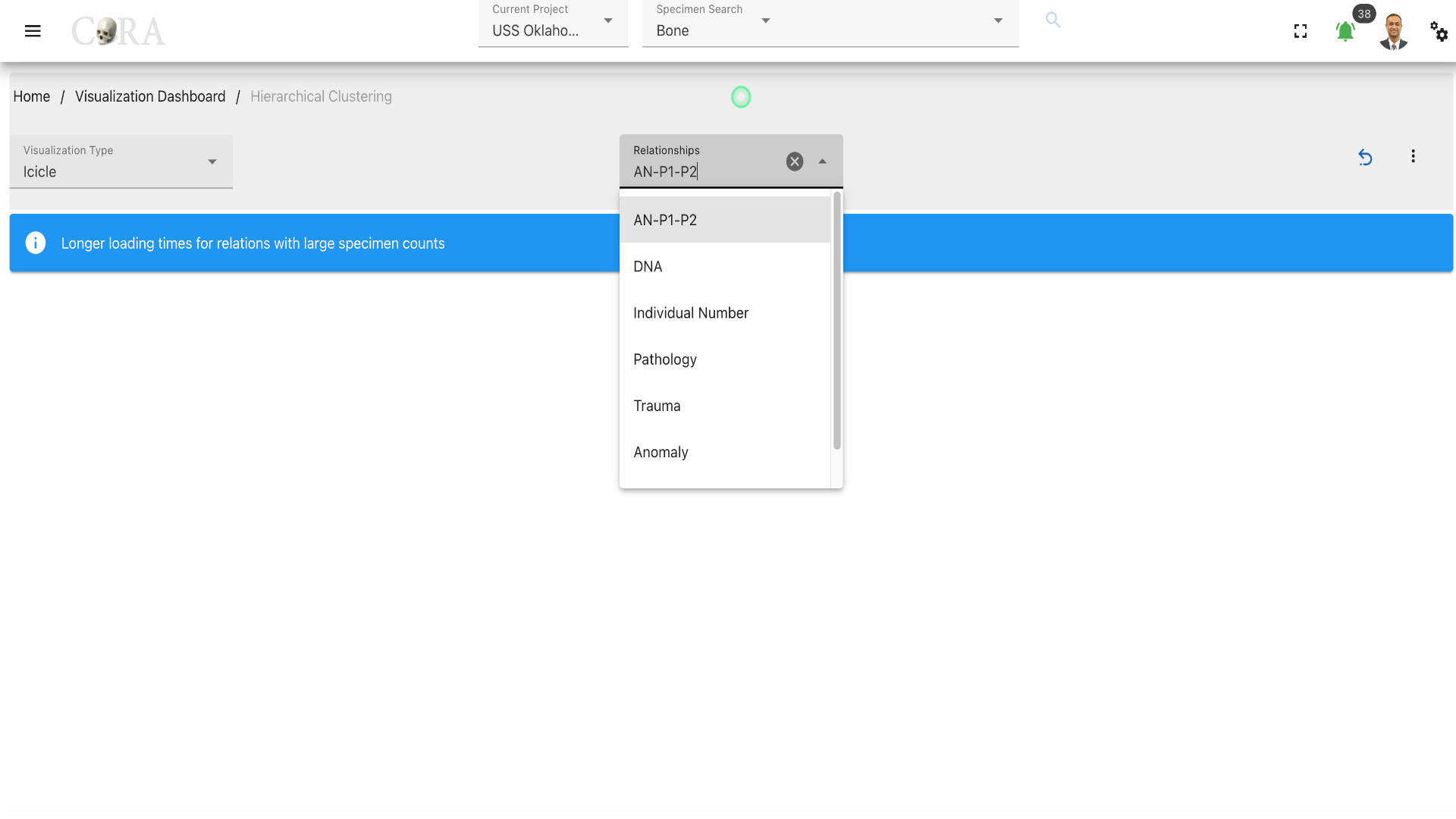
Select a relationship that is to be used in the hierarchical clustering.
Step-4: Visualization
After selecting the desired relationship the selected visualization is automatically generated. Each visualization type is interactive and can be changed until the desired output is achieved.
Different visualization types that are generated are shown below.
Icicle
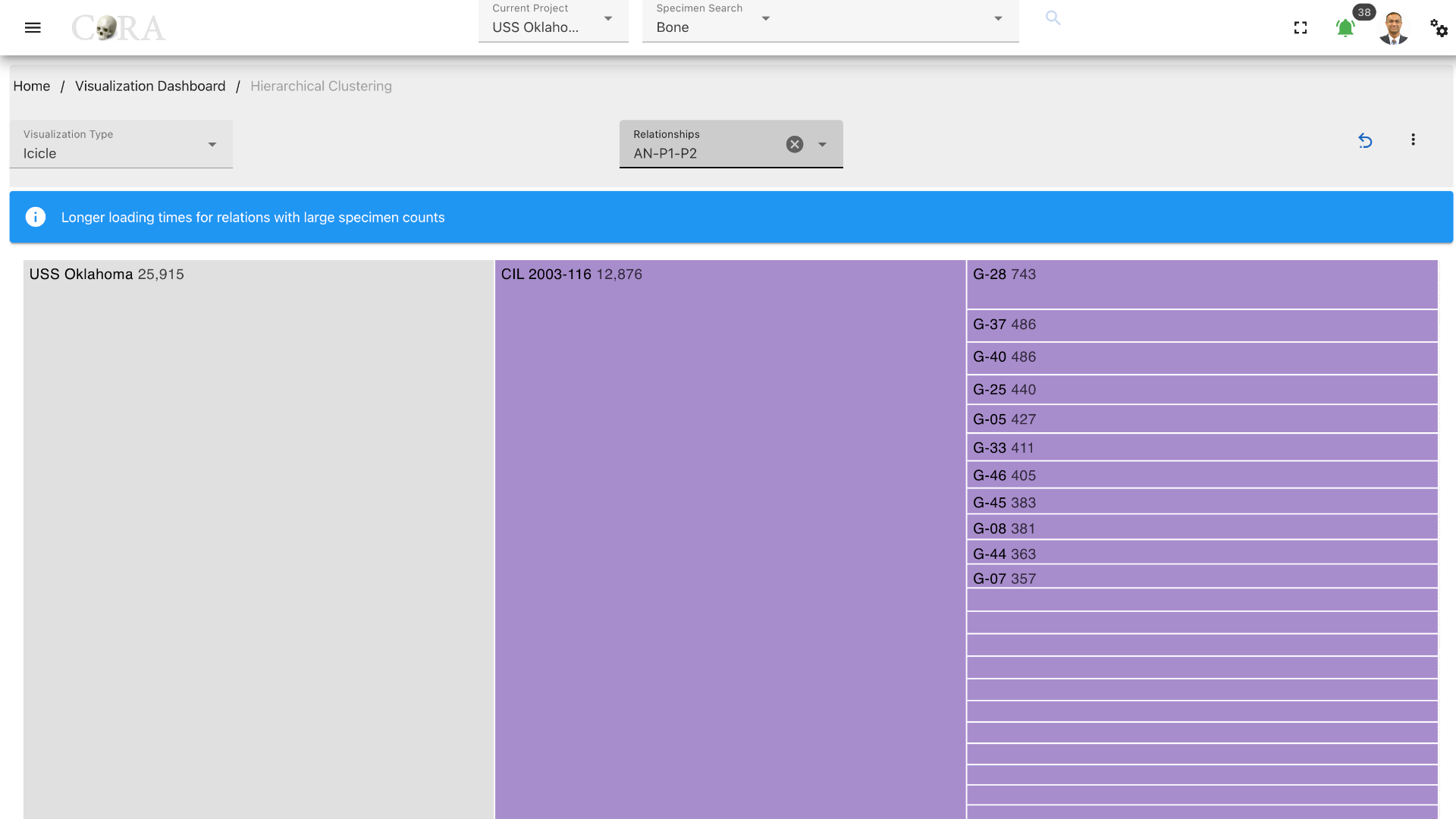
Treemap
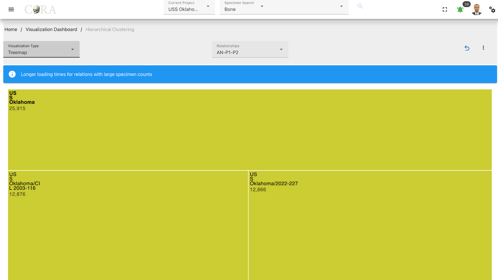
Sunburst
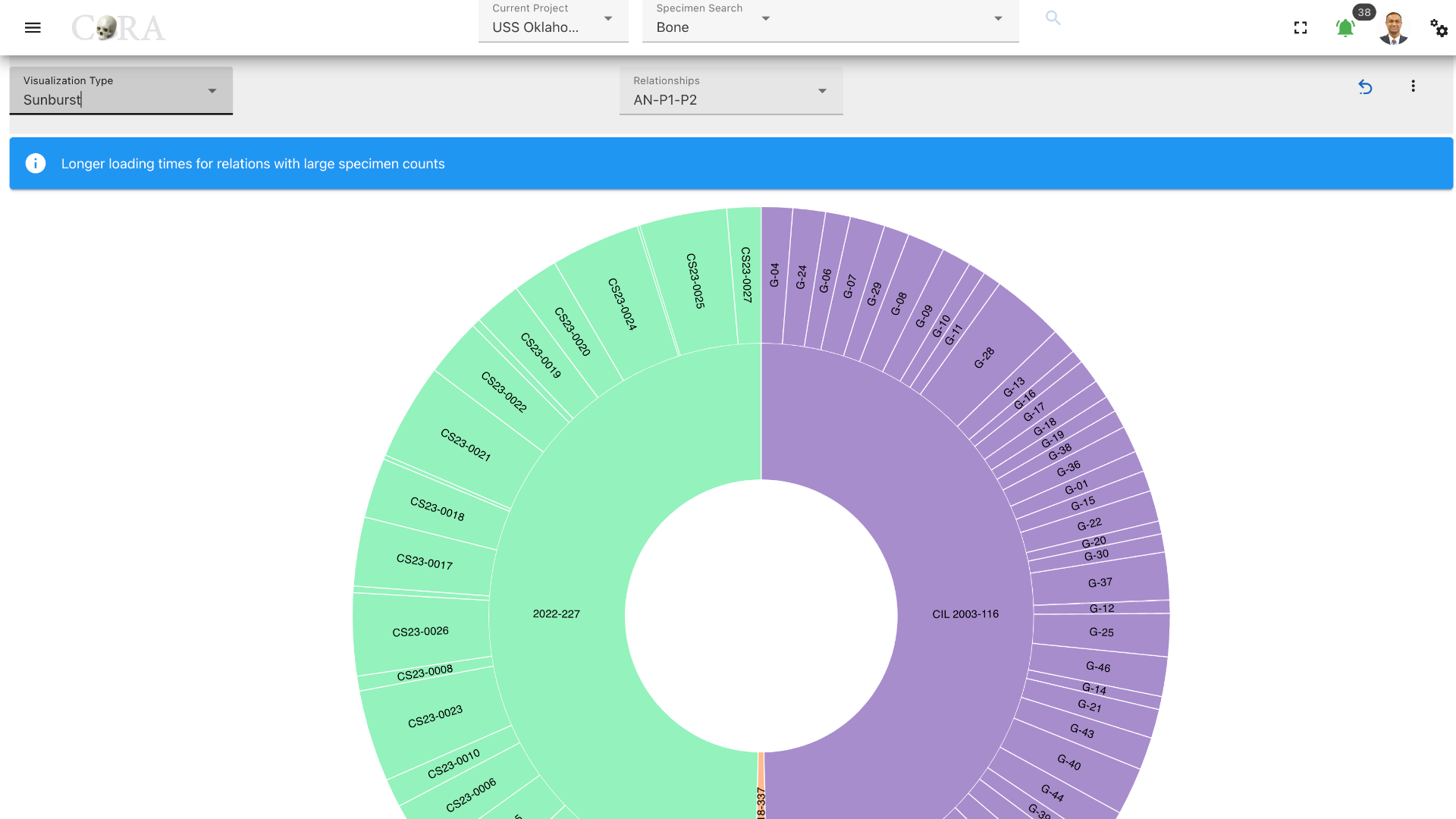
Circle Packing
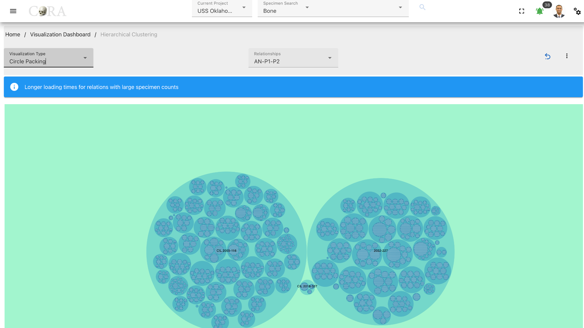
Indented Tree
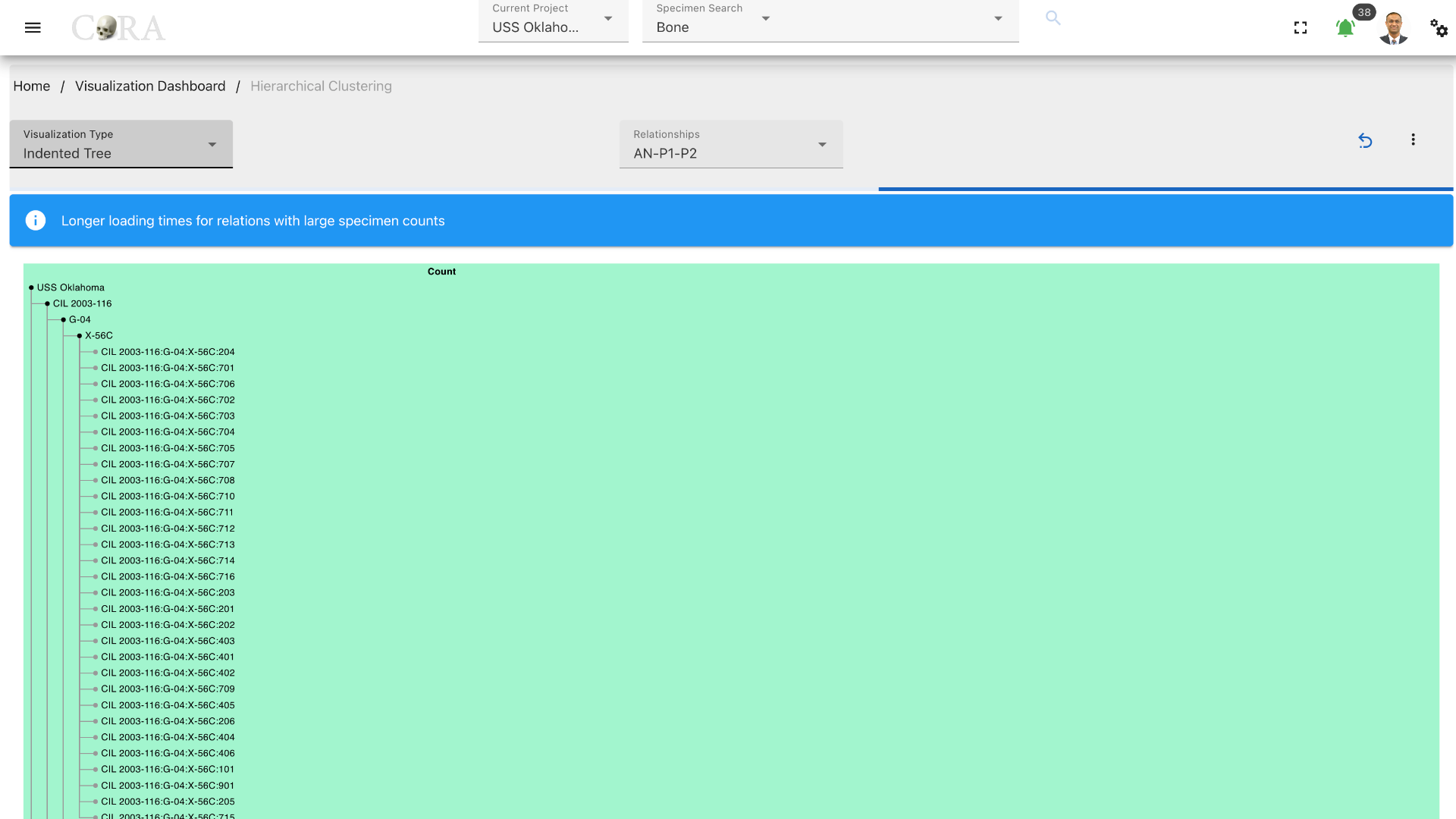
More Options/ Filters:
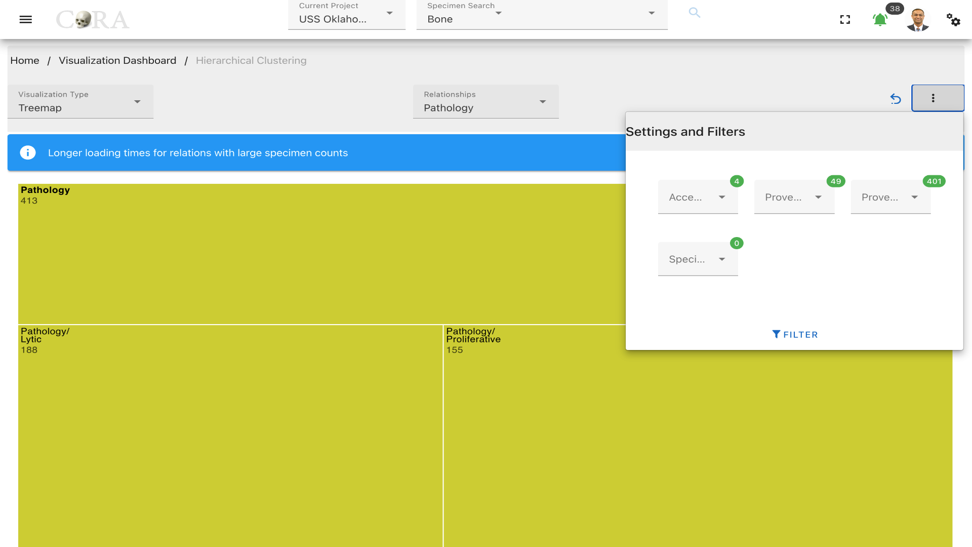 Click on the kebab menu in the top right corner to find more options. These options include filtering the specimens by
Accession Number, Provenance 1, Provenance 2 and a particular specimen can also be selected.
Click on the kebab menu in the top right corner to find more options. These options include filtering the specimens by
Accession Number, Provenance 1, Provenance 2 and a particular specimen can also be selected.
Hierarchical Edge Bundling
Hierarchical Edge Bundling
Hierarchical edge bundling is a visualization technique used to display complex networks of interrelated entities in a clear and organized manner. In CoRA, this method is used to illustrate relationships among different specimens within the dataset.
Each node on the perimeter represents a unique specimen, and the edges (lines connecting the nodes) represent relationships or associations between these specimens. The bundling of edges helps reduce visual clutter by combining multiple related paths into a single flow, making it easier to trace relationships within the hierarchical structure.
The following table shows the required and optional fields required for hierarchical edge bundling based on both relation and specimen.
Type: Relation
| Attributes | Required/Optional |
|---|---|
| Type | Required |
| Relation | Required |
| Type of selected relation | Required |
| Specimen | Optional |
Type: Specimen
| Attributes | Required/Optional |
|---|---|
| Accessions | Required |
| Provenance 1 | Required |
| Provenance 2 | Optional |
| Specimen | Required |
| Relation | Required |
Steps to generate Hierarchical Edge Bundle
Step-1: Select a type
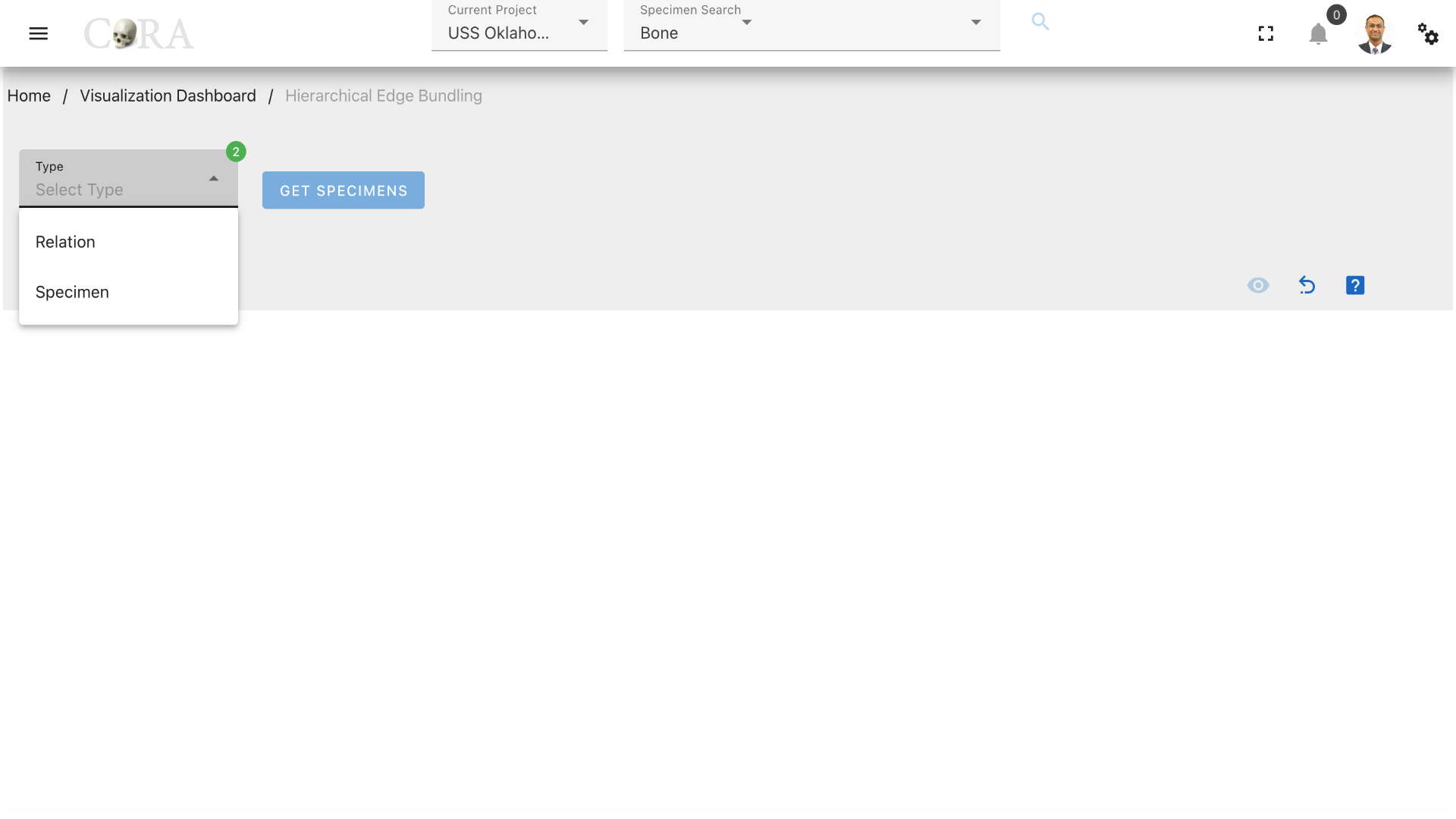
Select a type (relation or specimen) based on the requirement. Select 'Relation' if the hierarchical edge bundling has to be done based on the relations and its types associated with the specimens and select 'Specimen' if the hierarchical edge bundling needs to be done based a particular set of specimens.
Step-2: Select Relation
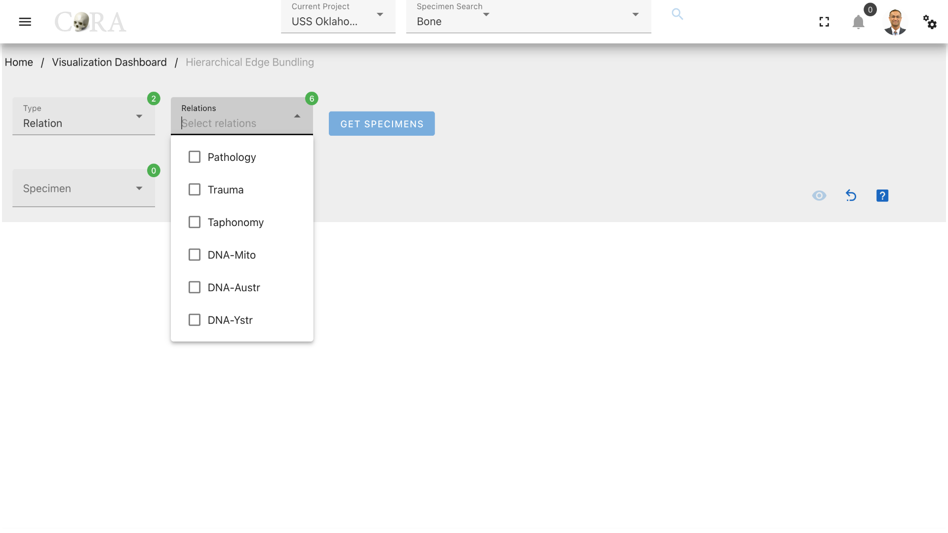
Select a relation associated to the desired specimens required for the hierarchical edge bundling. For example: Pathology
Step-3: Select a Pathology

Select a pathology or group of pathologies associated with the desired set of specimens and click on 'Get Specimens' to generate a list of specimens associated with the selected pathologies.
Step-4: Select specimens
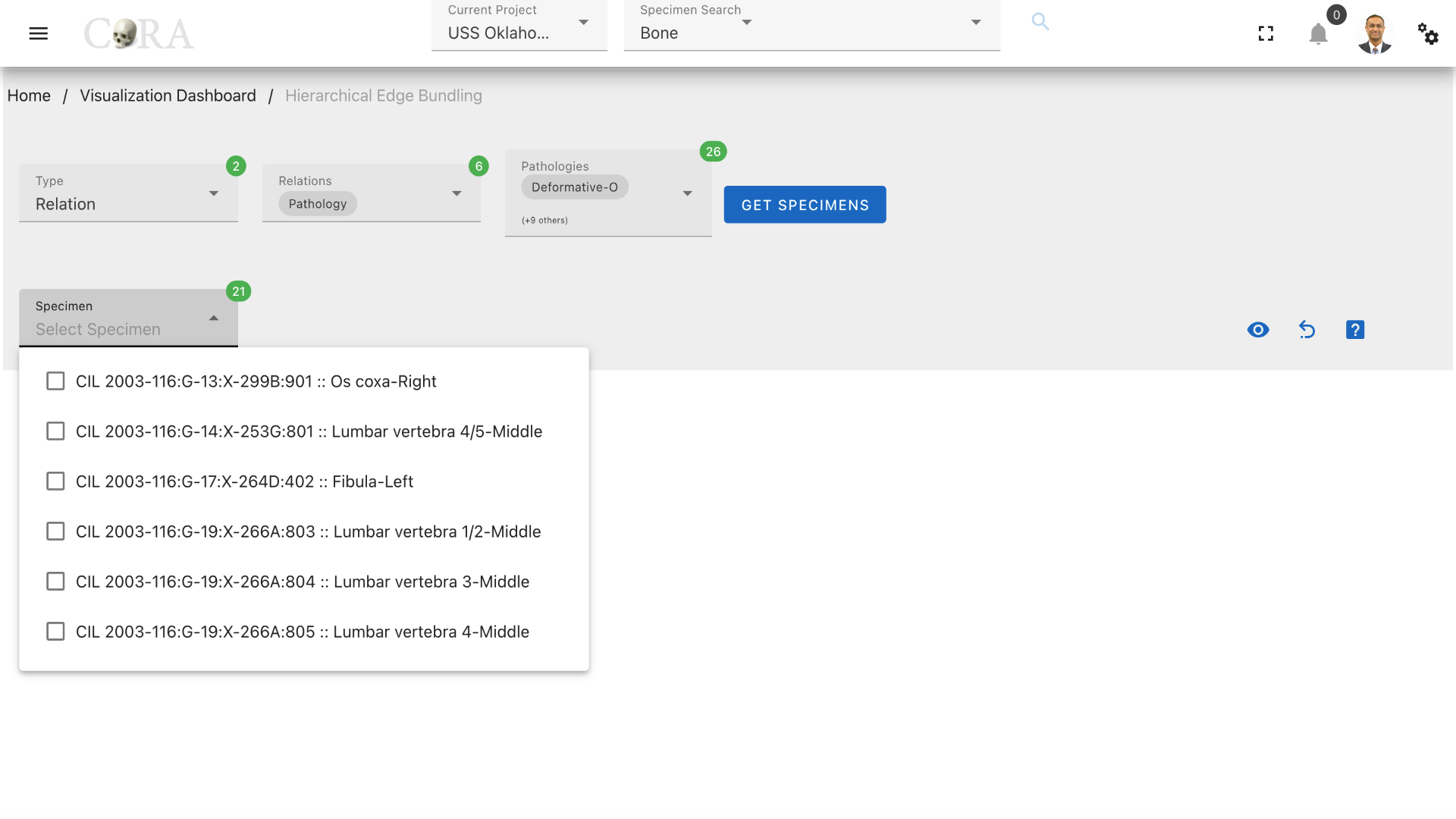
Select all the required specimens individually that are to be used for the hierarchical edge bundling or directly proceed to the next step to use all the available specimens.
Step-5: Generate the Hierarchical Edge Bundle
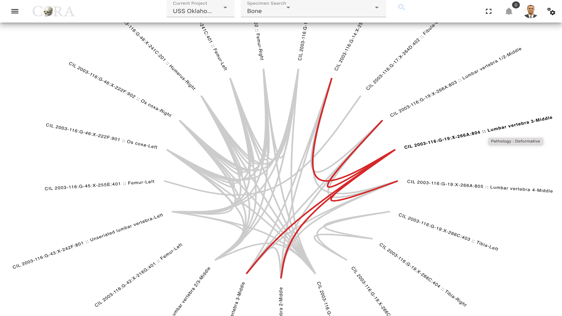
The Hierarchical Edge Bundle can be generated by clicking on the 'eye' icon for the selected specimens. Hovering over a specimen highlights a particular bundle of specimens which are associated with a similar type of pathology. Click on the 'reset' icon on the top to reset the page and try a new set of relations and specimens.
Measurement Scatterplot
Warning
This page is work in progress.
The measurements scatterplot can be used to narrow down your search space for likely pair matches. It can be used with any bones that allow for the capture of measurements such as Humerus, Ulna, Radius, Femur, Tibia, etc.
Note
Here is a complete list of bones measurements
Measurement Scatter Plot
A measurement scatter plot is useful for identifying or narrowing down for a given specimen which possible specimens are likely pair matches that deserve a more closer inspection
The following table shows the required and optional fields to generate a measurement scatter plot.
| Attributes | Required/Optional |
|---|---|
| Bone | Required |
| Side | Required |
| X-Axis Measurement | Required |
| Y-Axis Measurement | Optional |
| Specimen | Required |
Steps to generate a Measurement Scatter Plot.
Step-1: Select bone
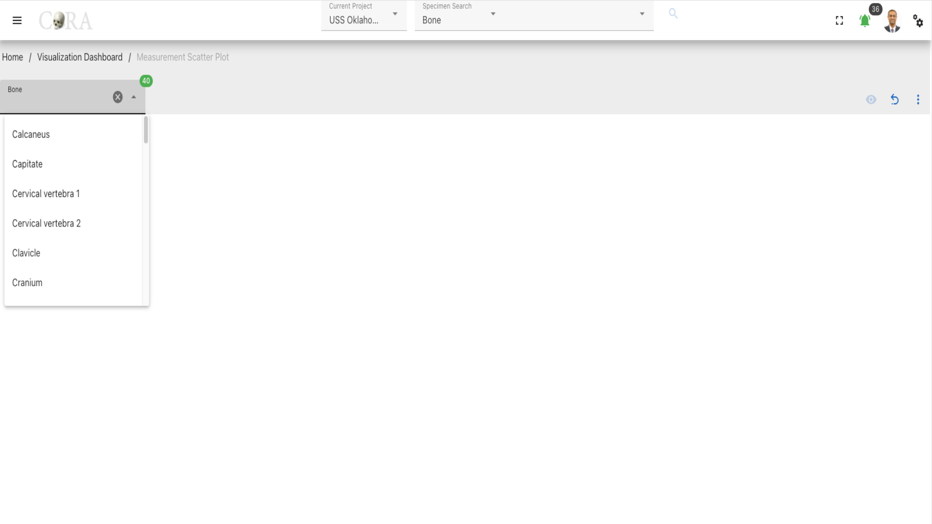 Select the bone type of the specimen from the available list of the bones required for the Measurement scatter plot generation and this will enable other field to show.
- Side
- X-Axis Measurement
- Y-Axis Measurement
Step-2: Select side
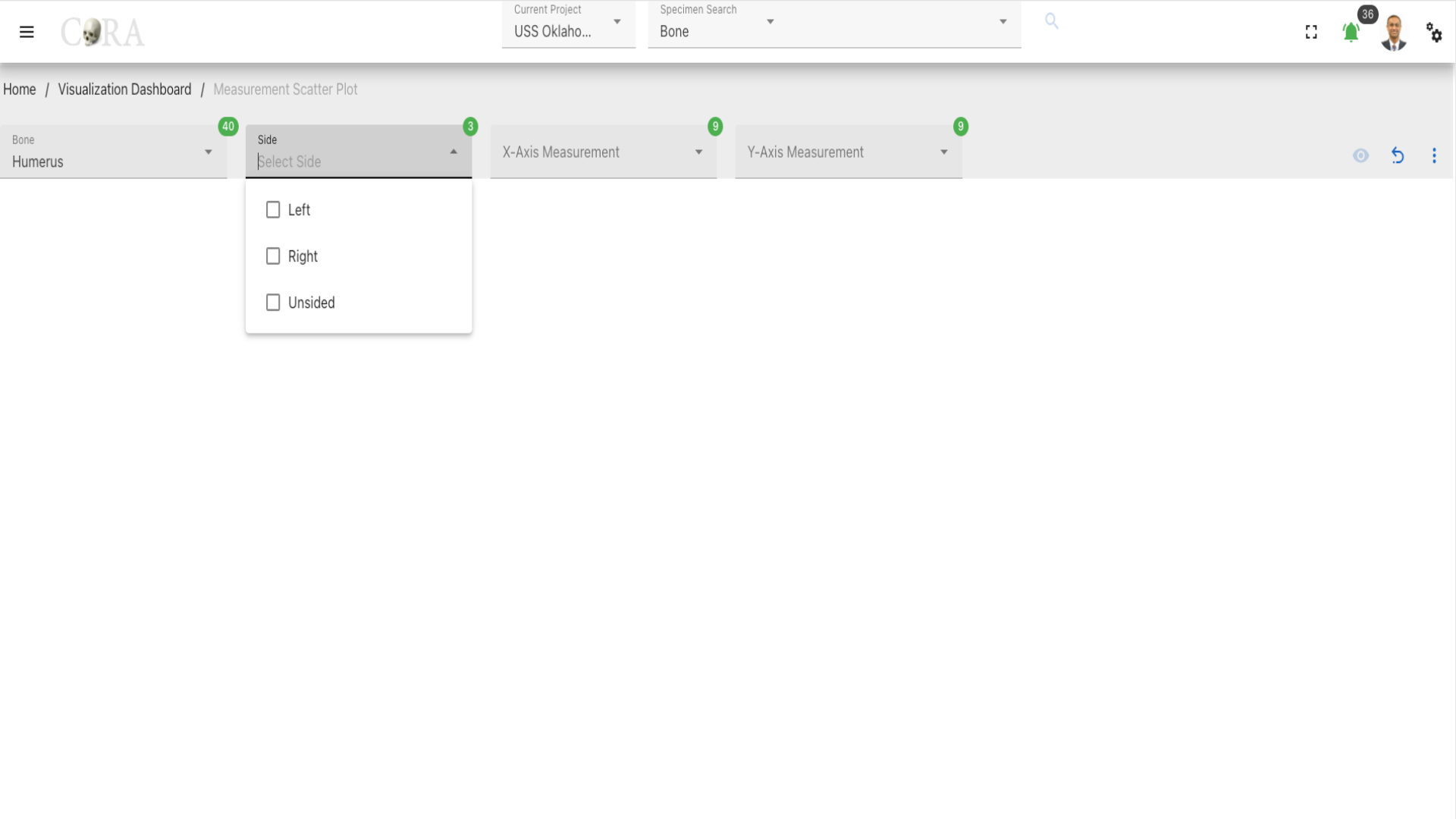 elect the Side to march the bone and the specimen from the available list of the sides. The following are the list of Sides available:
- Left
- Right
- Unsided
Step-3: Select X-Axis Measurement
Select the X-Axis Measurement for the Scatter plot.
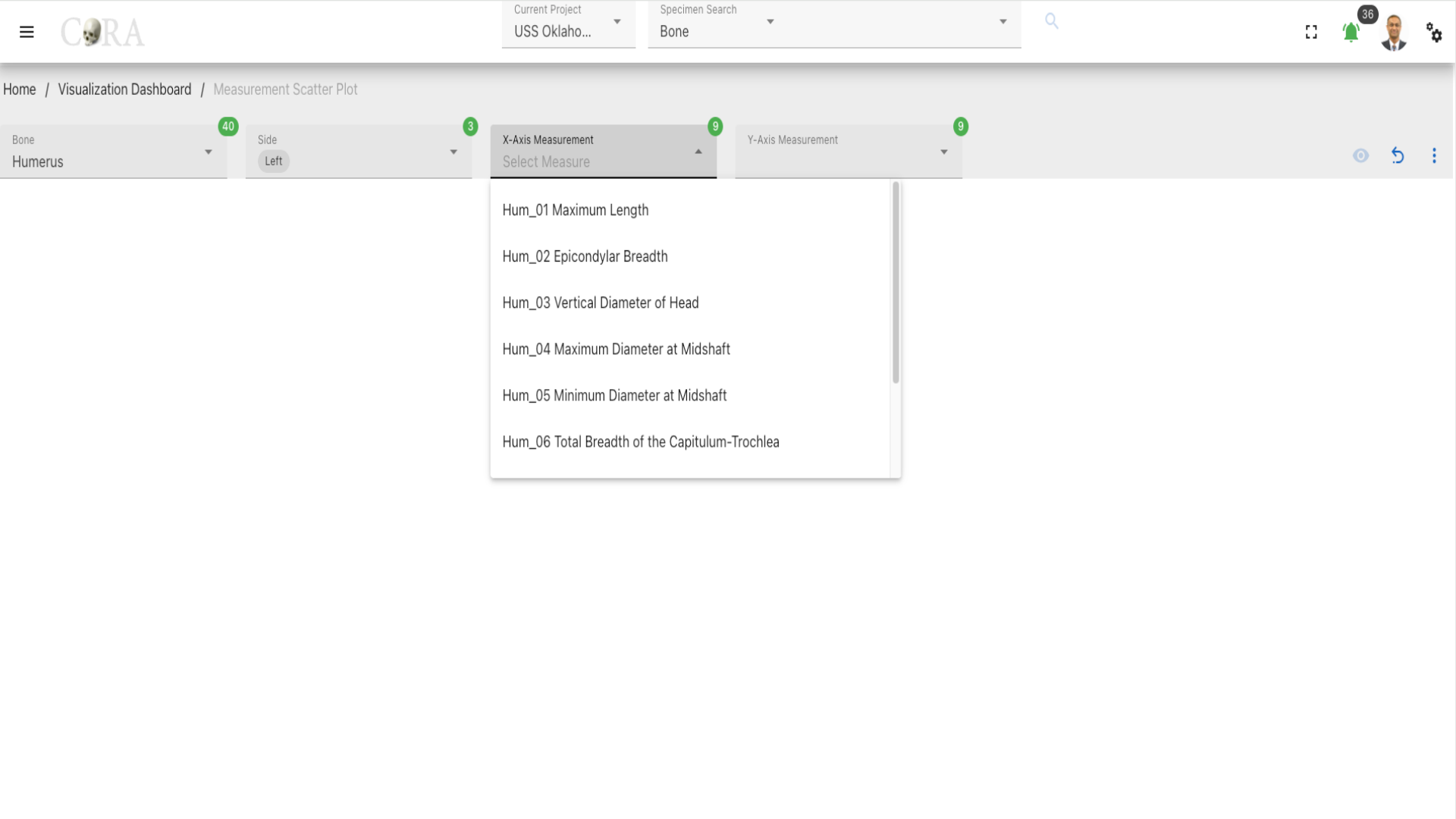
Step-4: Select Y-Axis Measurement
Select the Y-Axis Measurement for the Scatter plot, after selecting the Y-Axis Measurement proceed to click on the 'eye' to generate the scatter plot.
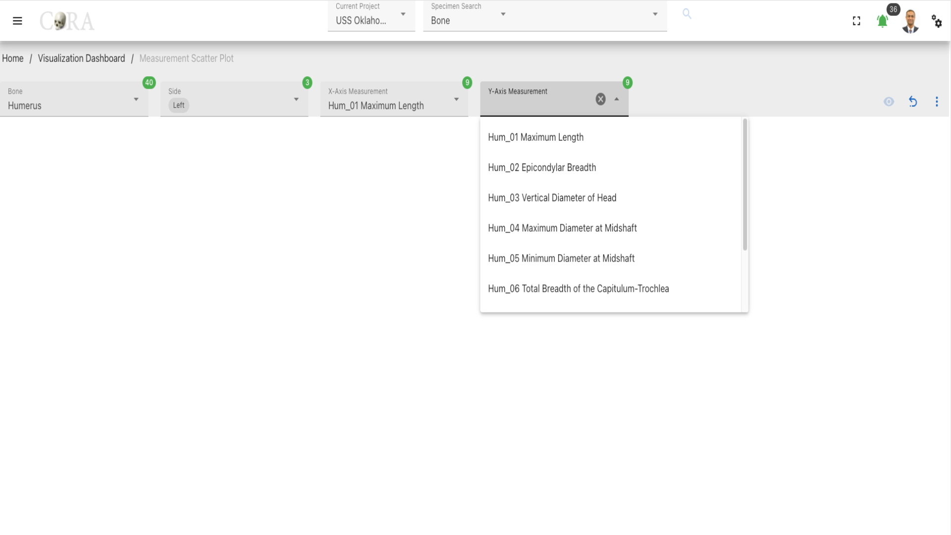
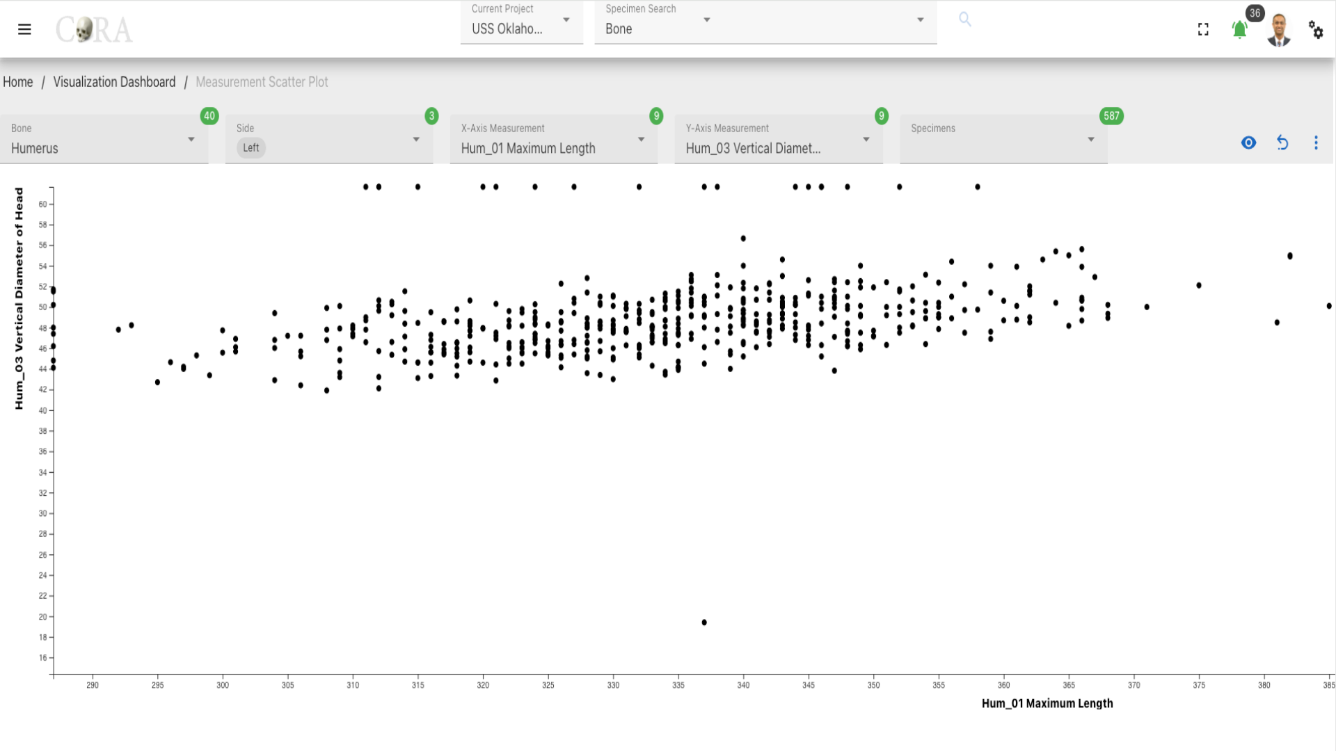
Step-5: Select a specimen
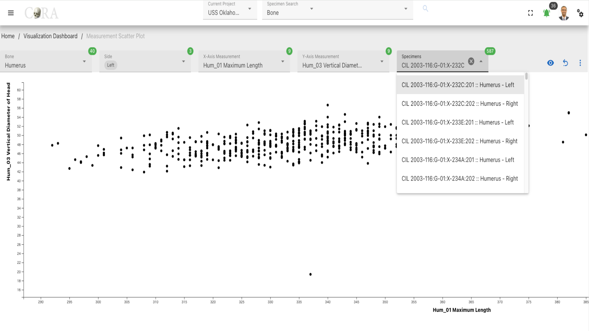
Select one or more Specimen based on the project requirement and click on the 'eye' icon to generate the visualization.
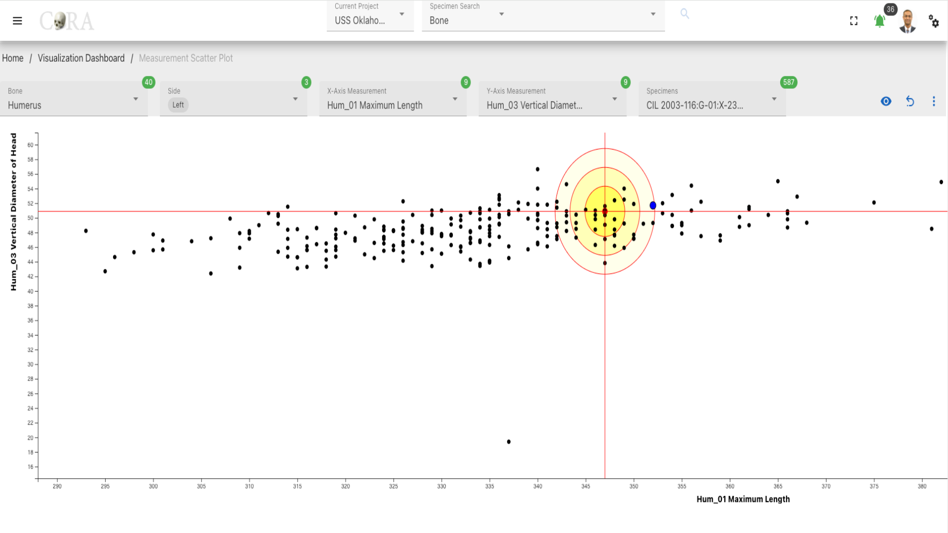
More Options/Filters
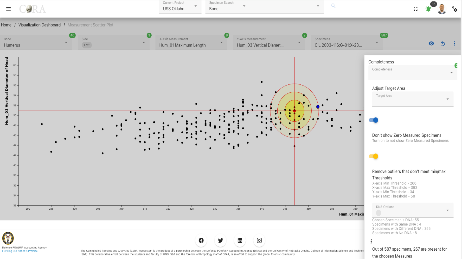 Click on the kebab menu icon to view more options to adjust the scatter plot to march the project requirement. The following are available when you click on the 'kebab'.
- Completeness
- Adjust Target Area
- DNA (Optional)
The bolded fields are selectable. - Don't show Zero Measured Specimens - Remove outliers that don't meet min/max - Graph Statistics Analysis - Graph Legend
Osteometric Sorting Regression
Warning
This page is work in progress.
Osteometric Sorting Regression
Osteometric Sorting Regression (OSR) is a statistical method used in the analysis of skeletal remains to sort and match bones based on their measurements.
The following table shows the required and optional fields required for osteometric sorting regression.
| Attributes | Required/Optional |
|---|---|
| Bone | Required |
| x-axis measurement | Required |
| y-axis measurement | Required |
| Specimen | Required |
Steps to use Osteometric sorting regression
Step-1: Select bones
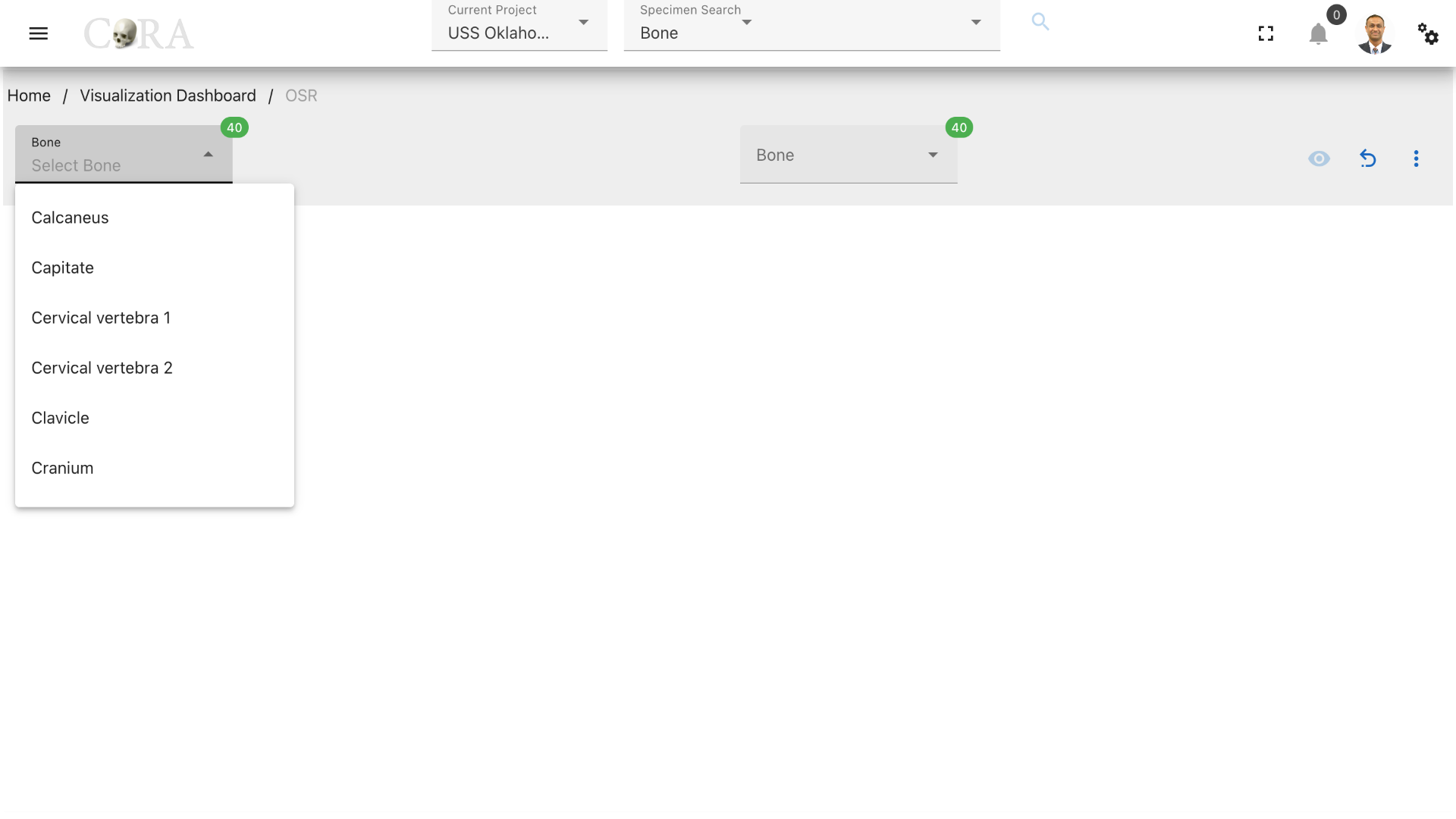
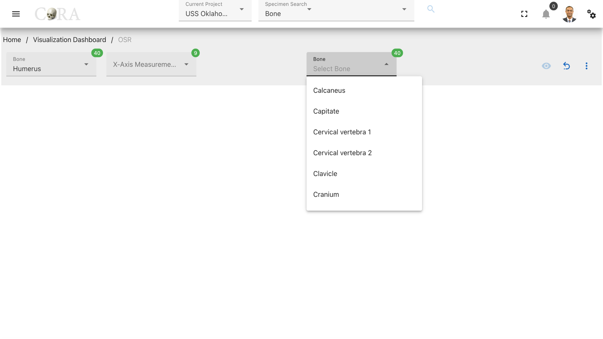
Select two bones from the two available dropdowns that are to be matched based on their measurements. (For example, Humerus and Tibia).
Step-2: Select x-axis and y-axis measurements
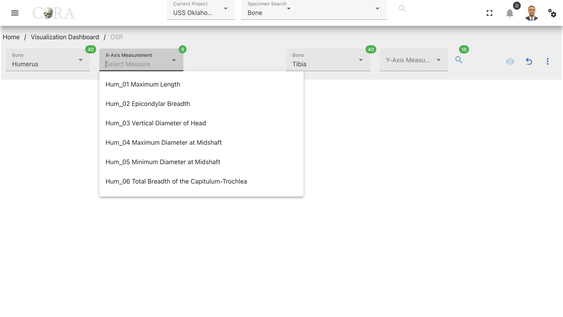
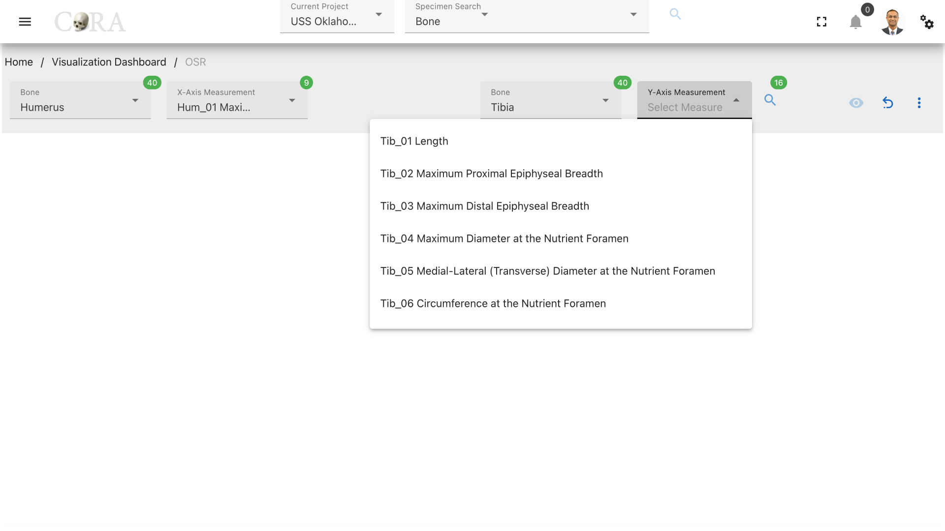
Select the x-axis measurement for the first bone and y-axis measurement for the second bone respectively. CLick on the search icon to generate a list of specimens (first bone type) with the selected x-axis measurement.
Step-3: Select a specimen
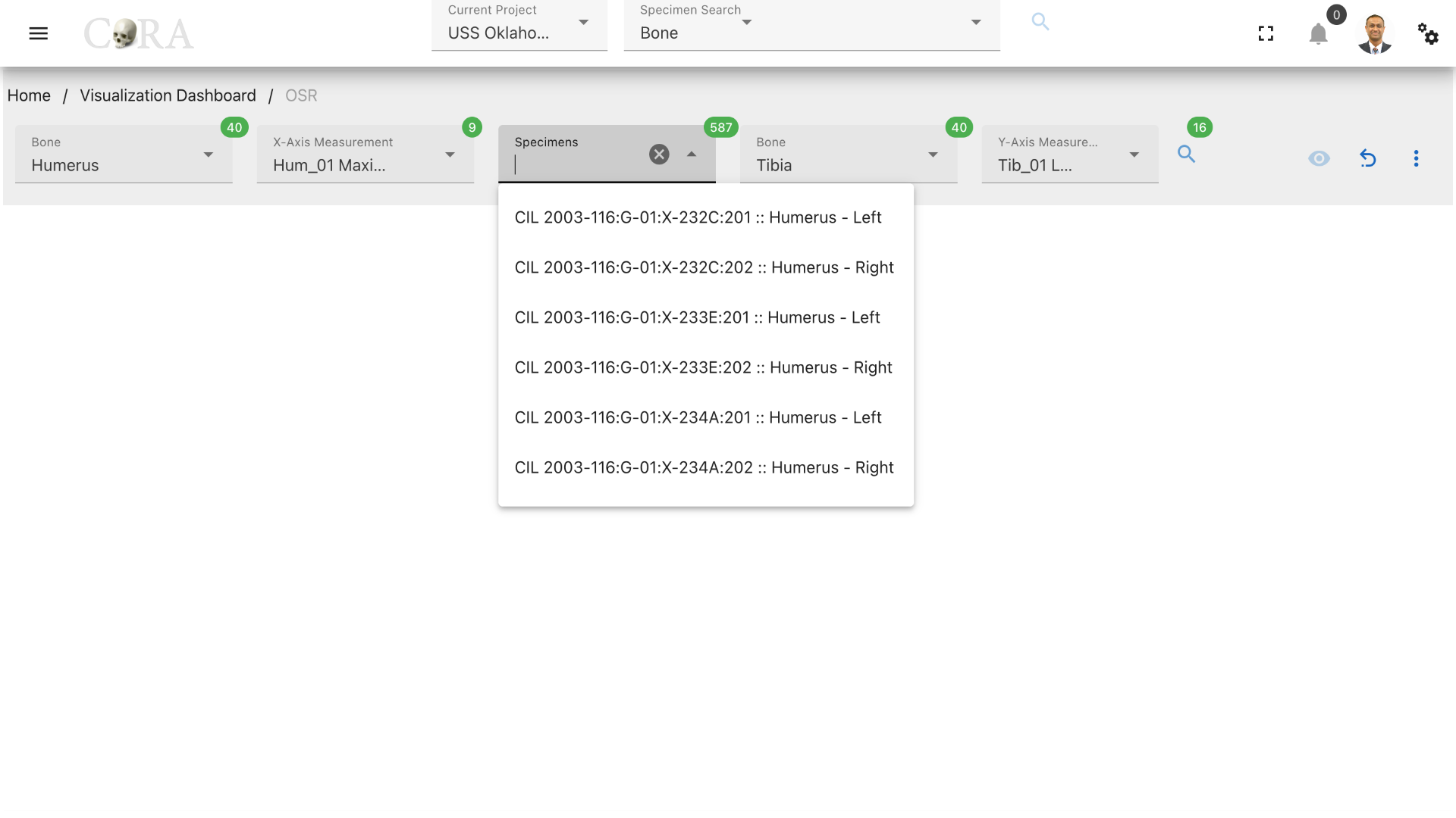
Select a desired specimen to be used in the sorting in order to find its match.
Step-4: Generate the Oseometric Sorting Regression Graph
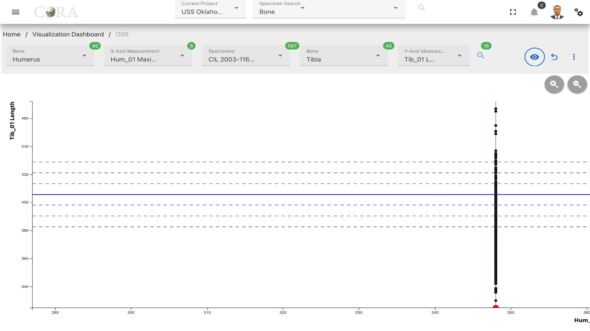
Click on the 'eye' icon to generate the osteometric sorting regression graph with the selected specimen highlighted in red.
More Options/Filters:
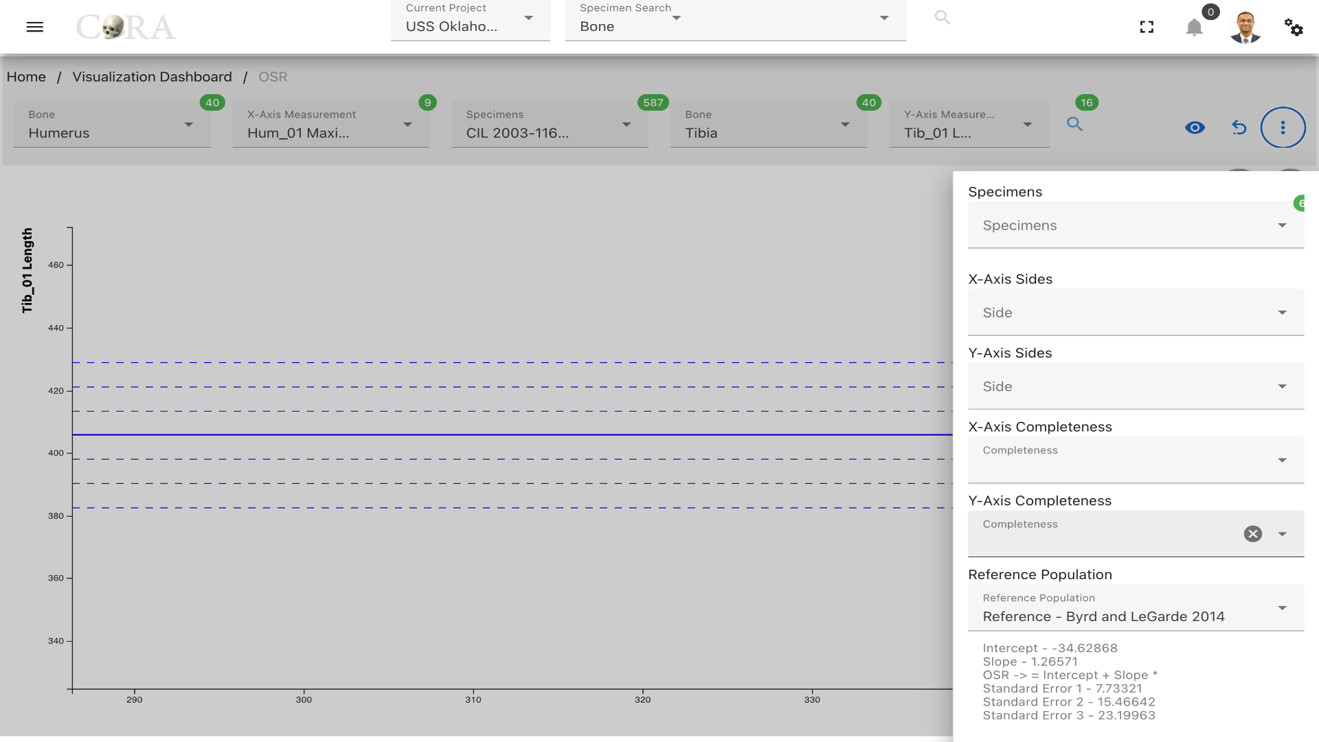
Click on the kebab menu to see more options. These options include - List of specimens for the second bone type that will be highlighted in blue when selected. - x-axis and y-axis bone sides and completeness to filter the specimens. - Reference population (Byrd and LeGarde 2014 selected by default). - Removing outliers that doesn't meet min/max thresholds. - DNA options (Specimens with same/different/no DNA) - Count of number of specimens available with the selected bone type and measurements.
Refits
Warning
This page is work in progress.
Refits Zone
Refits is a process used in osteological analysis where partial bones are attempted to be pieced/refit back together based on their physical fits and associations. This method is crucial for providing more complete skeletal reconstructions.
The following table shows the required and optional fields required for refits.
| Attributes | Required/Optional |
|---|---|
| Bones | Required |
| Completeness | Required |
| Side | Optional |
| Zones | Optional |
| Specimen | Optional |
Steps to generate Refit-Zones Visualization
Step-1: Select a bone
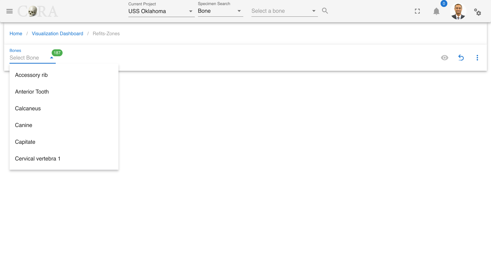
Select a desired type of bone that requires refits.
Step-2: Select Completeness
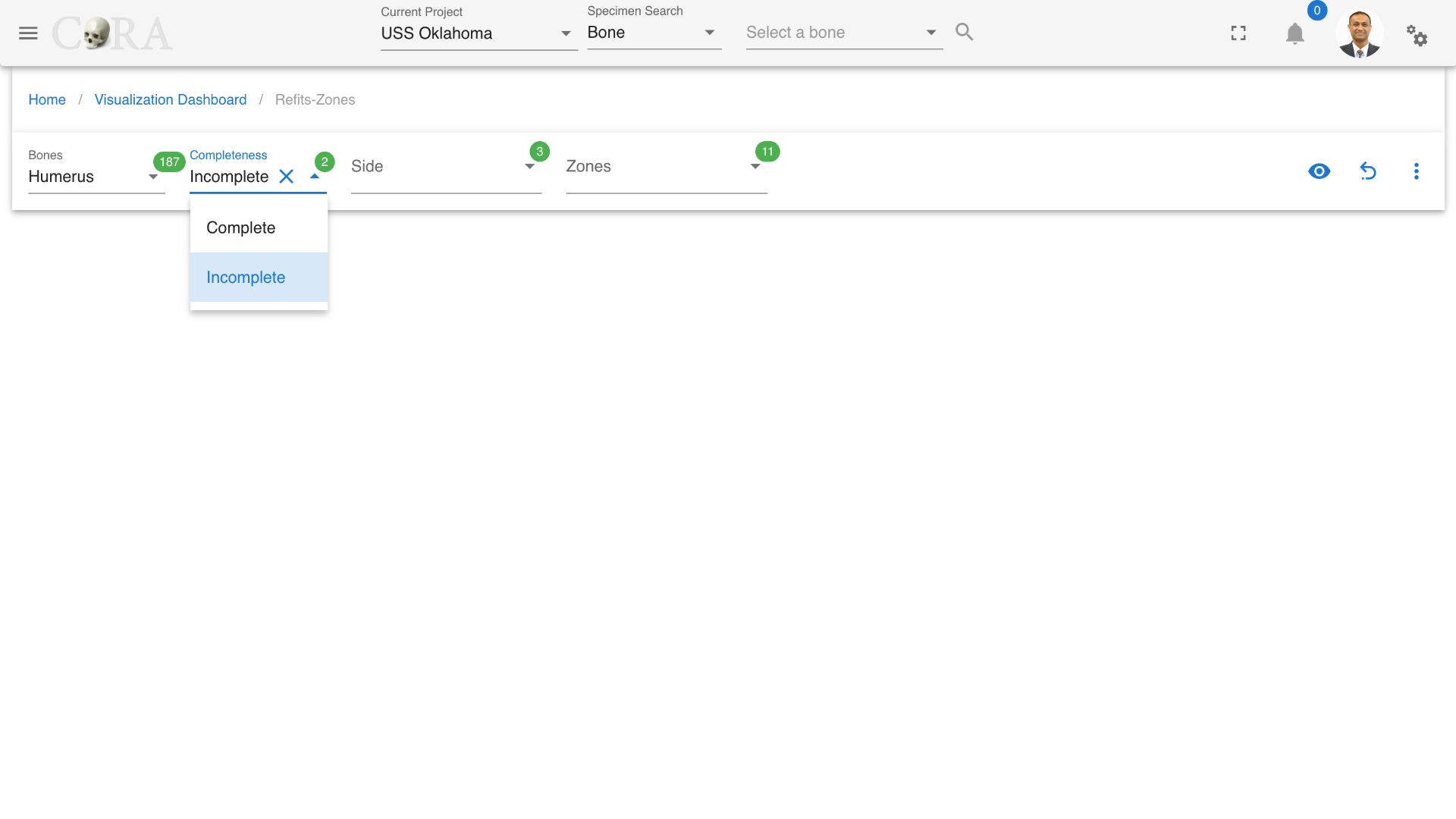
Completeness of a bone is set to incomplete by default as incomplete bones are the ones that need refits.
Step-3: Select side of the bone
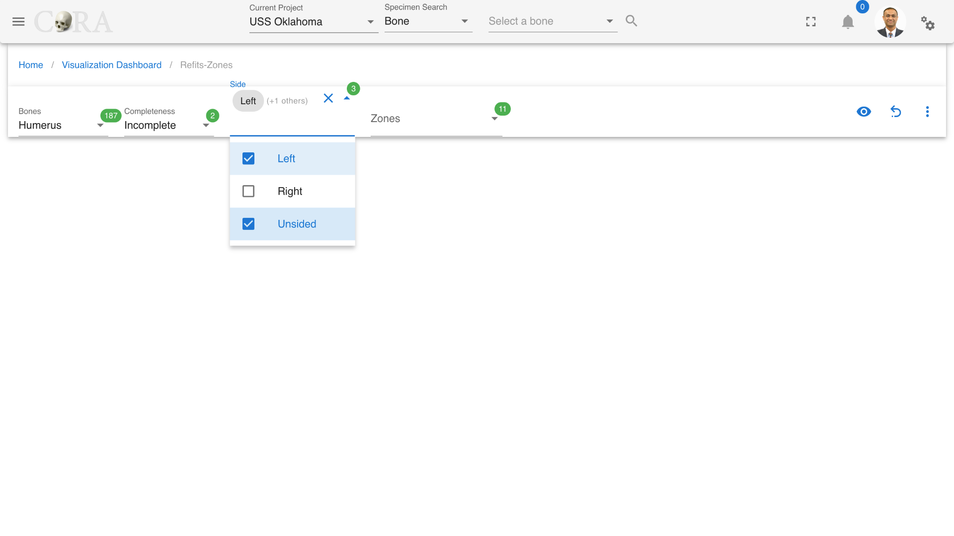
Select appropriate bone side that requires refits.
Step-4: Select zones
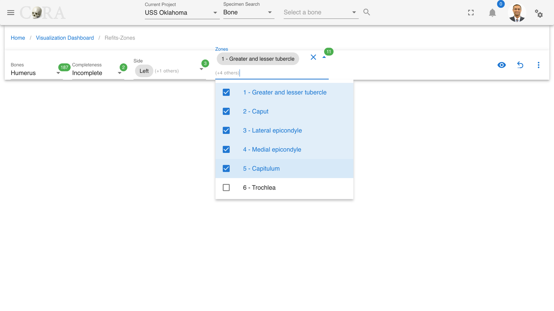
Select a single or multiple zones from the list of available zones that will be highlighted in the graph.
Step-5: Generate the refits visualization
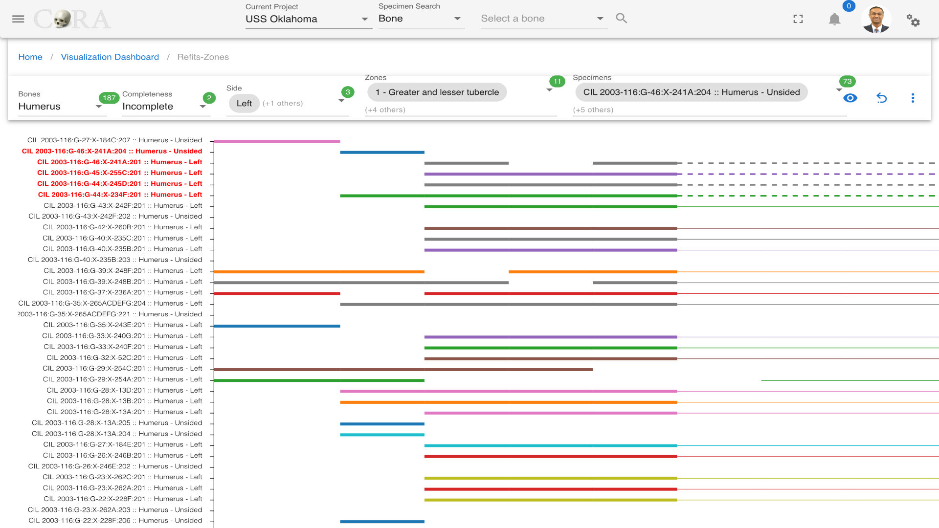
Click on the 'eye' icon to generate a graph with all the relevant specimens and their refit zones. Under specimens select specimens to highlight them in red and find a fit to them.
More Options/Filters:
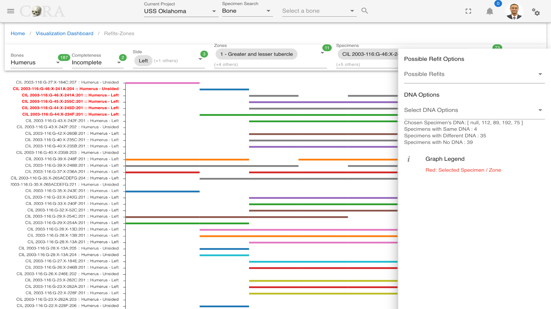
Click on the kebab menu icon to view more options. These options include - Possible refit options and - DNA Options (Specimens with same/different/no DNA)
Possible Refit Options
In the menu on the right side, you can see more possible refits options on how your refits-zone display.
This field can be multi-select - Exact Refits - Exact Refits Multiple - 1-Overlap - 2-Overlap - 3-Overlap
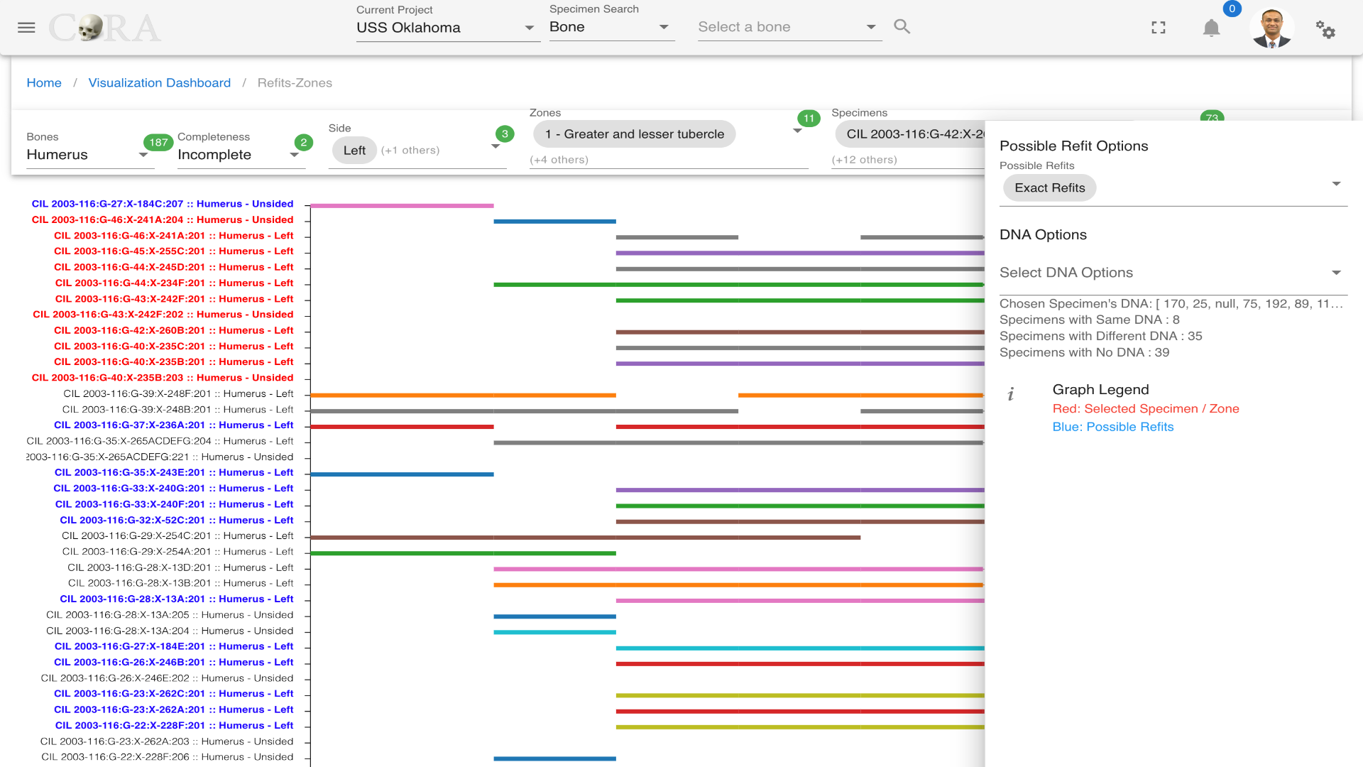
For possible refit options, for example, if we select exact refits all the possible refits will be highlighted in blue.
Use the 'reset' button to reset the graph and generate a new one.
Relationships graph
Single/multiple Relationship Graph
The Single/Multiple Relationship Graph is a type of visualization used to illustrate complex relationships between a central node and multiple related nodes, which may themselves interact with one another or with additional nodes.
The following table shows the required and optional fields to generate a single multiple relationship graph.
| Attributes | Required/Optional |
|---|---|
| Graph Type | Required |
| Relation | Required |
| Specimen | Optional |
Steps to generate a single/multiple relationship graph

Step-1: Select graph type
 The graph type is always defaulted to force directed graph and no change is required.
Step-2: Select a relation.

Select a relation from the list of available relations. For example: Pathology.
Step-3: Generate the graph
 Click on eye icon to generate the single/multiple relationship graph.
Step-4: Choose a specimen
 Choose a desired specimen that will be highlighted in the graph.
More Options/Filters:
 Click on the kebab menu to find more options. These options include
- Filtering the specimens by Accession number, Provenance 1 and Provenance 2.
- Choosing subtypes in relations. (For example: Types of pathologies)
- Disjoint graph toggle
Stature Estimation
Note
This page describes how to perform and visualize stature estimation using different anthropological methods in the CoRA platform.
Accessing Stature Estimation
From the left navigation:
Left Sidebar Menu → Visualizations → stature Estimation
This section enables users to estimate the stature of an individual using specific skeletal remains and reference methods.
Select Parameters
Use the filter bar at the top of the page to configure your input:
- Individual Numbers: Select the unique ID of the individual (e.g., CIL 2003-116-G-01).
- Specimen: Choose a specific bone specimen associated with the individual.
- Methods: Select a stature estimation formula (e.g., Trotter and Gleser 1952-WF).
- Unit: Choose the measurement unit (inches or centimeters).
- Precedence Order: Toggle to apply the precedence order.

This module estimates the likely height of an individual based on bone measurements and selected forensic estimation formulas.
Two Approaches to Stature Estimation
Approach 1: Single Specimen
- Select:
- Individual Number
- Specimen
- Method
-
Unit (inches or centimeters)
-
Click the (eye icon) to generate a visual representation of the estimated stature based on the selected single specimen.
-
The result appears in the Visualization tab, showing:
- Skeleton aligned to a height chart
- Height estimation banner (e.g.,
± 67.97 inches)

This approach is ideal for quick, visual insights using one specific bone.
Approach 2: Specimens in Individual
- Select:
- Individual Number
- Method
-
(Leave specimen unselected)
-
The system automatically uses all associated specimens for the selected individual.
-
Results: A - Visualization tab shows the average stature estimation.

Best suited for comprehensive analysis across all available skeletal data for an individual.
B - Stature Calculations tab shows the formulas, calculations, maximum, minimum, average Height for all the specimens of the selected specimen. - Indivudal number - Specimen key - Method name - Equations - Measurement of each specimen - Minimum, Maximum, and Average height for the individual

- Precedence Order
The Precedence Order checkbox allows users to prioritize the order of specimen usage.

- Enabling this option will:
- Automatically arrange specimens according to the precedence hierarchy.
- Affect both the visualization and calculation outputs.
- Ensure consistency in methods that rely on preferred bone types.

Use this feature when you want consistent and scientifically prioritized height estimations based on bone type.
Interface Overview
Filter Panel Options
- Individual Numbers: e.g.,
CIL 2003-116-G-01 - Specimen: (Optional for aggregated view)
- Methods: e.g.,
Trotter and Gleser 1952-WF - Unit: Inches or Centimeters
- Precedence Order: Toggle to apply bone prioritization.
Visualization Tab
Displays a visual skeleton aligned with a height chart based on selected method.
Stature Calculations Tab
Provides a tabular view of:
- Indivudal number
- Specimen key
- Method name
- Equations
- Measurement of each specimen
- Minimum, Maximum, and Average height for the individual
This module supports detailed forensic reporting and anthropological research by leveraging scientifically validated height estimation models.
Knowledge Graphs
Knowledge Graphs
The CoRA analytics engine provides the ability to leverage advanced analytics using project specific knowledge graphs. The CoRA knowledge graphs leverages the Neo4J Graph database to allow forensic anthropologists and scientists to better understand & analyze their project specimens and its related data to help in the missing persons identification process. It allows forensic scientists to find relationships between specimens using related data such as DNA, pair matching, articulations, taphonomy, anomaly, trauma, pathology, among others.
So What is a Knowledge Graph?
A knowledge graph is a design pattern for storing, organizing, and accessing interrelated data entities, including their semantic relationships. With knowledge graphs, you can better understand your data and build more intelligent applications. A knowledge graph contains three essential elements:
- Entities, which represent the data of the organization or domain area.
- Relationships, which show how the data entities interact with or relate to each other. Relationships provide context for the data.
- An organizing principle that captures meta-information about core concepts relevant to the business.
Here is the process guide that project leads and their teams can use to get access to their projects knowledge graph DBMS.
Please note that advanced analytics using knowledge graphs are worked on at a regular basis to fine tune their performance. Please consider these to be in experimentation phase until final release. You are encouraged to use the advanced analytics using knowledge graphs as is.
Info
We would appreciate your use of these advanced analytics using knowledge graphs and your feedback on making them better and more useful to you. Thank you.
Project Canvas
Project Analytics Canvas
The Project Canvas is a powerful interface for managing specimen assignments to individuals in forensic anthropology cases. It provides a visual, drag-and-drop workflow for linking skeletal elements to identified individuals based on anatomical, DNA, and association data.
Access and Layout
- Open the main navigation by clicking the Hamburger Menu (three horizontal lines) in the top-left corner.
- Select Project Canvas under the Analytics & Visualization menu from the navigation menu.
- On the Project Canvas page, select your Individual from the Individual Lab Table using the dropdown menu.
- The dropdown displays individual identifiers (e.g.,
CIL 2003-116-I-110.1). - You can search within the dropdown by typing to filter the list.
![]()
The Project Canvas header contains several action buttons in the top-right corner. Each icon serves a specific function:
| Icon | Name | Description/Functionality |
|---|---|---|
| Specimens Lab Table | Show and Hide the Project Specimens & their associations Lab table | |
| DNA Lab Table | Show and Hide the DNA Specimens & their associations Lab table | |
| Individual Lab Table | Show and Hide the Project Individuals & specimens Lab table | |
| Info Tip | Provides contextual information/tips about the current page | |
| Help - CoRA Docs | Opens the contextual help page in CoRA Docs for the current page. |
![]()
Lab Tables
The Project Canvas consists of three main Lab tables arranged horizontally, namely the Individuals, Specimens and DNA Lab Tables. Each Lab table serves a distinct purpose and contains specific filtering, sorting, and data display capabilities.
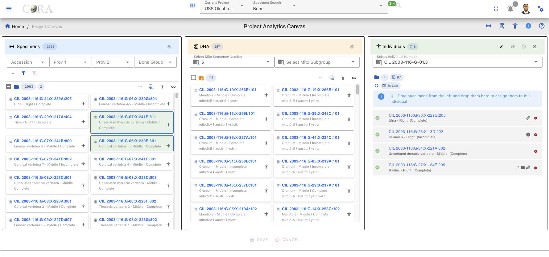
Lab Table Buttons/Icons
| Icon | Description |
|---|---|
| DeDup or Removes duplicate records from DNA Associations that already exist in DNA. | |
| Displays the hop/degree association and visualizes specimen connections for the chosen hop. When the icon is clicked, a hop can be selected from a dropdown list. The system displays all records up to the selected hop. Hovering over a hop number shows the hop number and its associated specimen information. | |
| The first number is count of specimens on table. The second number is count of selected specimens (highlighted with a green background). | |
| Filters specimens unassigned to an individual. light grey (unassigned), dark grey (all specimens) | |
| Highlights associations between DNA and DNA Associations. When enabled, associations are clearly shown. When disabled, DNA Associations are outlined with a red dashed border to remain visible when a DNA specimen is selected. | |
| Auto select all specimens in lab table | |
| DNA mito sequence number does not match with DNA mito sequence number on selected individual | |
| DNA mito sequence number matches with DNA mito sequence number on selected individual | |
| Toggle selected specimens only |
Specimens Lab Table
The Specimens Lab table can displays all skeletal elements/specimens available in the current project. But it is recommended that you use the search filters to reduce your search space and only pull in the specimens that are required for the current task. Once you pull in specimens on to the lab table it will display the count fo the specimens for the current filters.
Search and Filtering
- Located at the top of the lab table
- Allows searching by specimen Accession, Provenance1, Provenance2, Bone Group, Bone, Individual Number, Side and Completness
- For expansion and advanced filtering, Click the Expand Arrow (chevron) below the filter row to reveal additional filtering options:
- After completion,click the blue filter icon underneath the filter bars to execute.
- Reset All (Red Icon) button clears all filters at once.
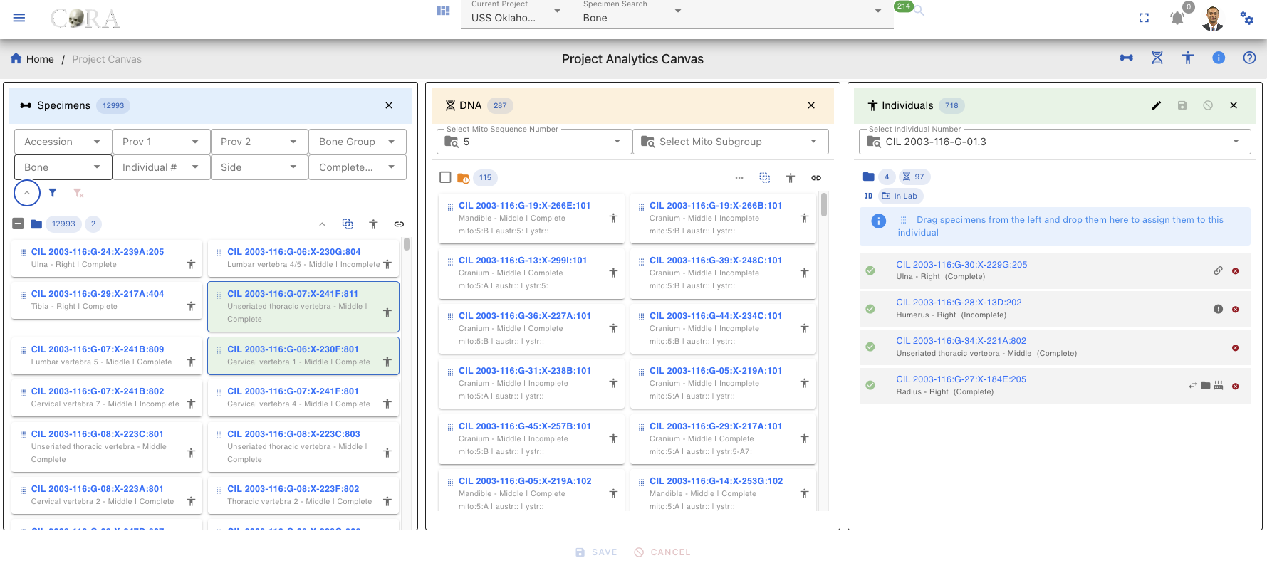
Specimens Card
Each specimen in the list appears as a card containing:
- Specimen key (e.g., CIL 2003-116:G-07:X-241B:805)
- The key is clickable to jump to the specimen page where you can view details such as Accession Number, Bone, Side, Designator, etc.
- Link Icon (chain link symbol) - Located on the specimen card, click to open the Specimen Associations Lab Table
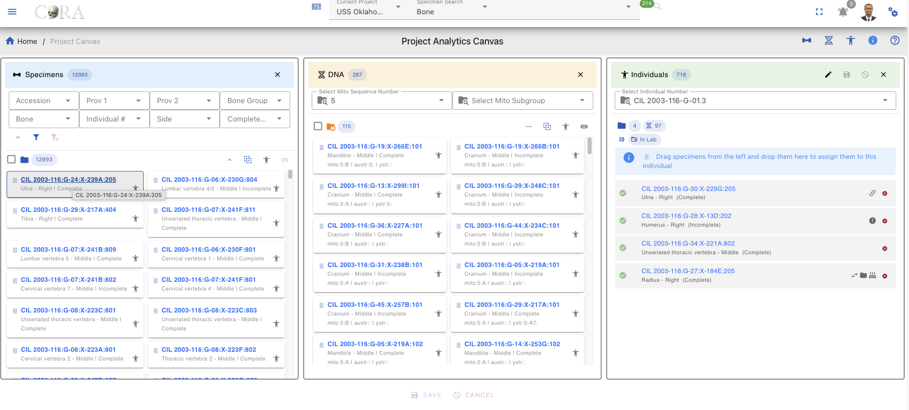
Specimen Page View
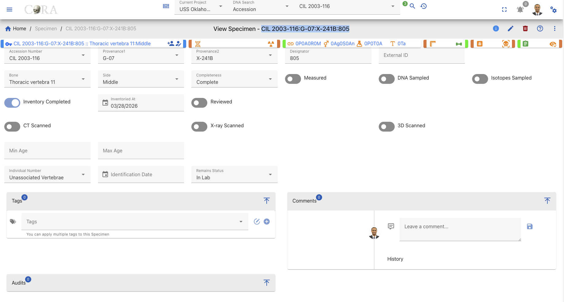
Specimen Associations Lab Table
After clicking the Link Icon (chain link) on a specimen card in the Specimens Lab Table, a new Associations compartment/popup appears. This compartment provides detailed association information for the selected specimen.
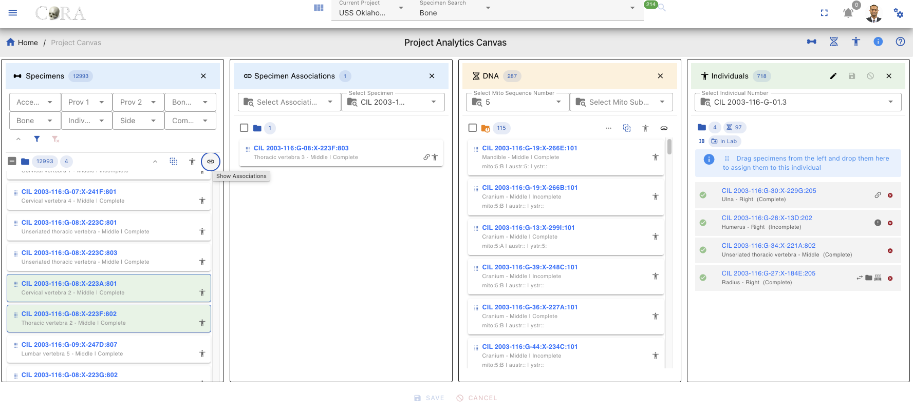
Association Filters
The lab table includes an Association Type dropdown filter that allows you to view specific types of associations
| Filter Type | Icon | Description |
|---|---|---|
| Articulations | Shows only Articulation specimen | |
| Pair | Shows only paired specimens (e.g., left and right bones) | |
| Refits | Shows only refitted fragments that rejoin to form a complete element | |
| Morphology | Shows only morphological matches (similar morphological features) |
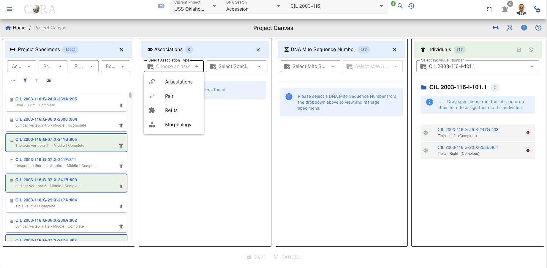
Association List
Once filters are applied, the corresponding Specimen or DNA association lab table displays:
- The key of each specimen type
- Underneath the specimen key Bone Name, Location and Status
- Right side of the specimen key Type of Relation, Human Icon
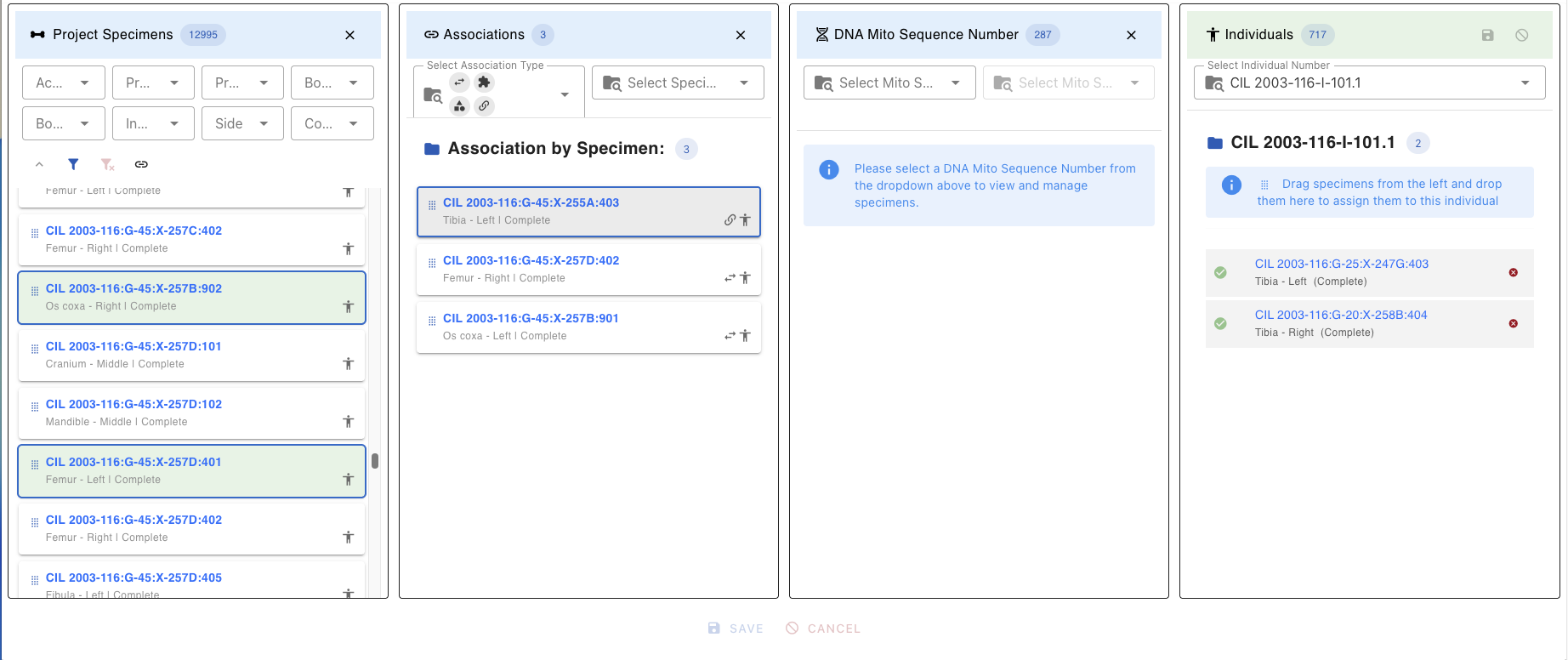
Association Close
To close the Associations lab table click the X button in the top-right corner of the lab table
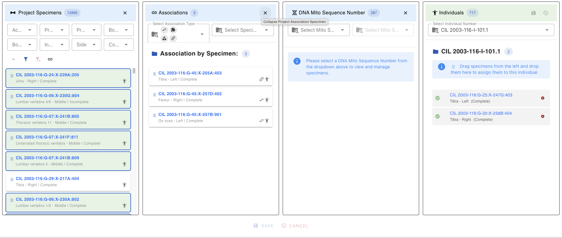

DNA Lab Table
The DNA Lab table displays all DNA Mito Sequences available in the current project. Selecting a DNA Mito Sequence number will pull in all specimens with that mito sequence number and their associatiosn that are 1 Hop/Degree from them. Once you select a DNA Mito sequence number the lab table will display the count fo the specimens for the current sequence number.
Mito Sequence Number
The primary filter is a dropdown search containing all unique mito sequence numbers in the project: - Click the dropdown to see all available sequence numbers - Search within dropdown: Select to filter the list of sequences - The selected Mito Number appears in the header with the records filtered to that sequence.
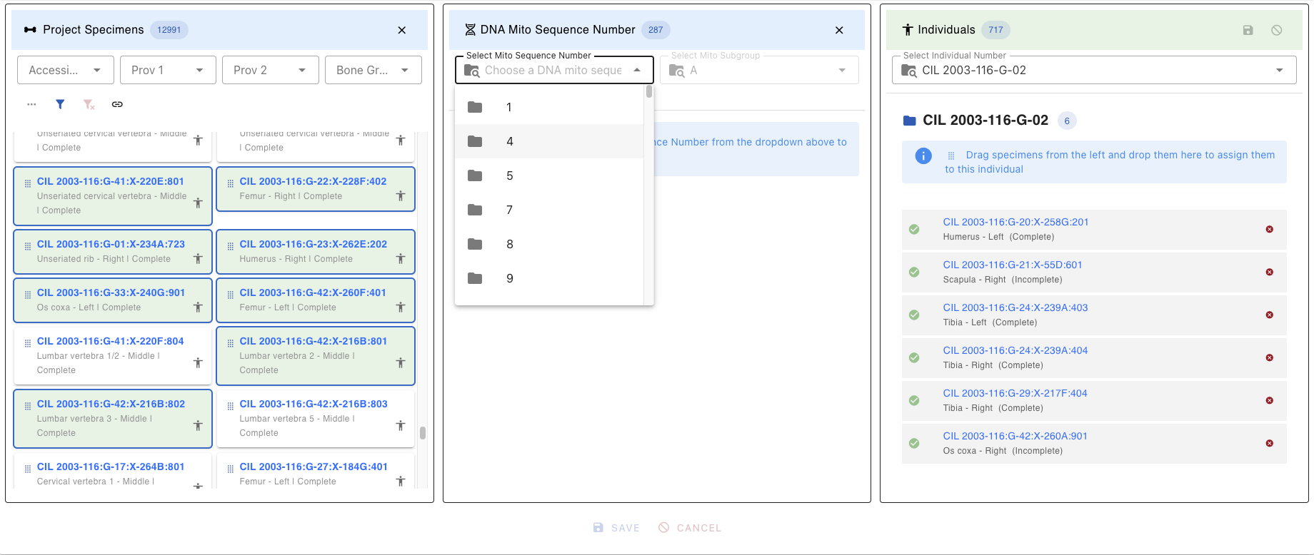
Filters
Once a mito sequence is selected
- The DNA Lab table automatically filters to show only specimens with matching DNA mito sequence number
- Specimens are grouped or highlighted by their genetic relationship
- The DNA Association Lab table updates to show existing associations for filtered specimens
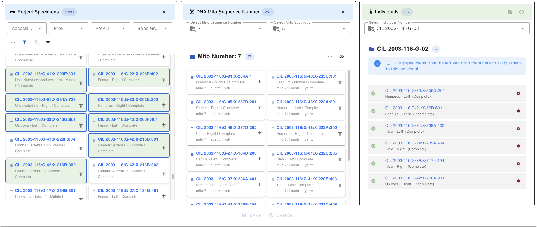
DNA Lab Specimen Card
Each specimen in the DNA Lab Table appears as a card containing
- The key of each Mito Sequence Number(e.g.,
CIL 2003-116:G-07:X-241B:805) - Underneath the Mito Sequence Number key Bone, Side, Completness, Sequence Number
- Right side of the specimen key Human Icon
- Link Icon (chain link symbol) - Located on the DNA Lab Table, click to open the DNA Associations Lab Table
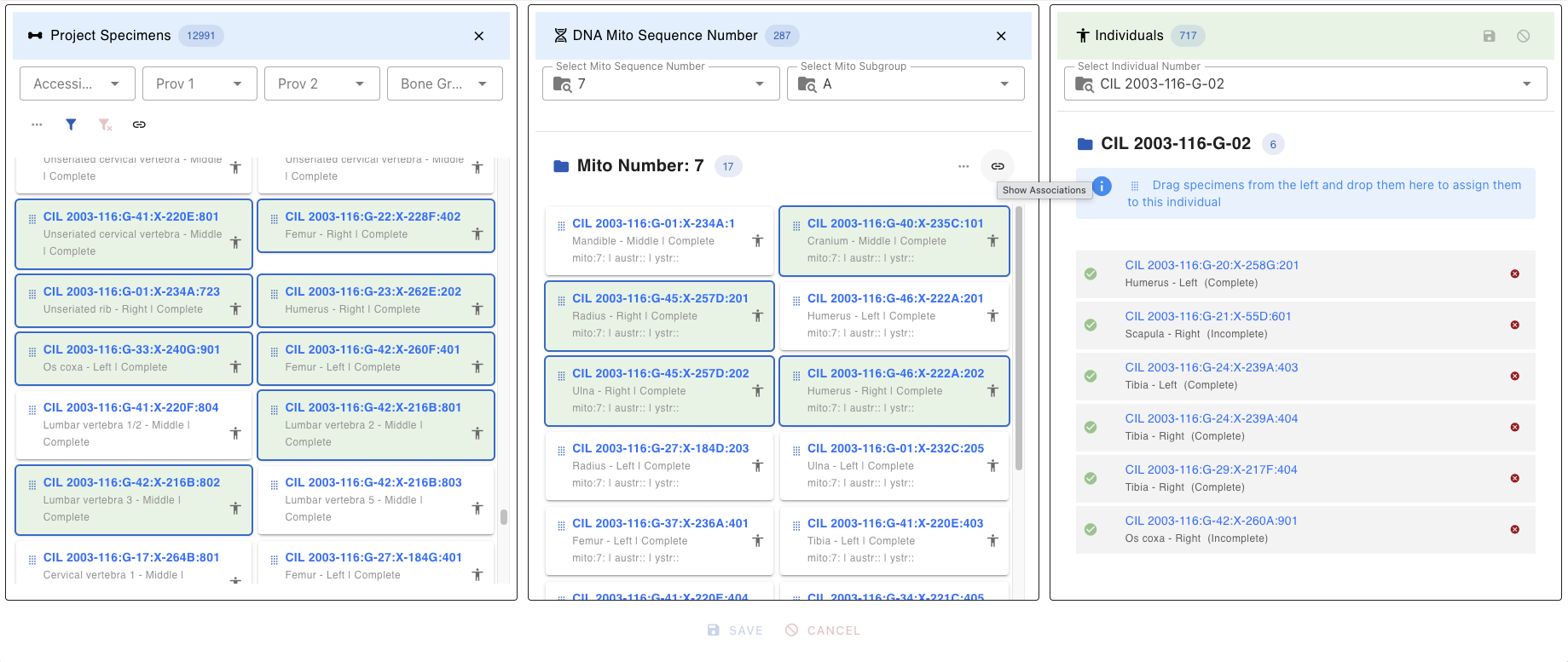
(Screenshot: DNA Mito Sequence dropdown with search functionality) specimen card click , card view
DNA Association Lab Table
After clicking the Link Icon (chain link) on the DNA Lab table, the DNA Associations lab table will be displayed. This DNA Associations Lab table provides detailed association information for the selected specimens.
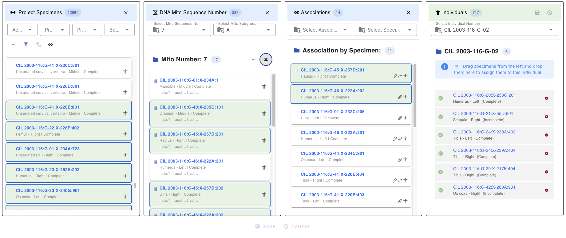
Selecting Association Chain
Whenever a specimen is selected in the DNA Associations Lab table, it automatically selects the corresponding DNA specimen in both DNA Lab table and DNA Associations Lab table.
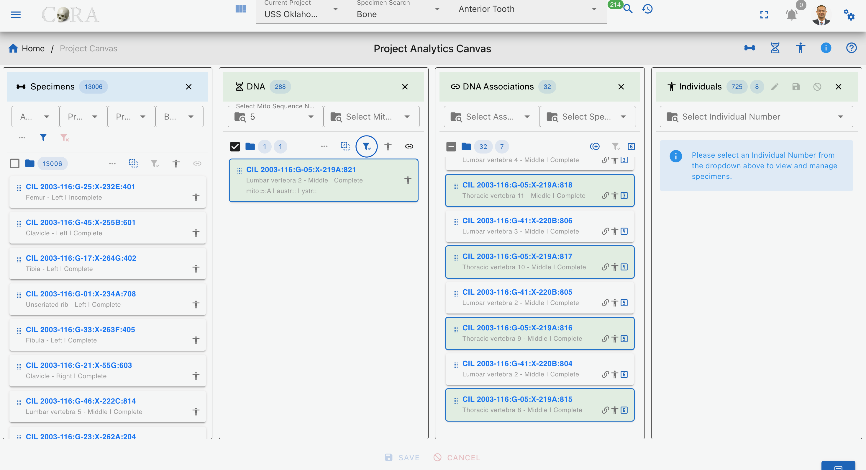
When we hover over the hop number, it shows the hop number and its root parent and immediate parent information (to be implemented).
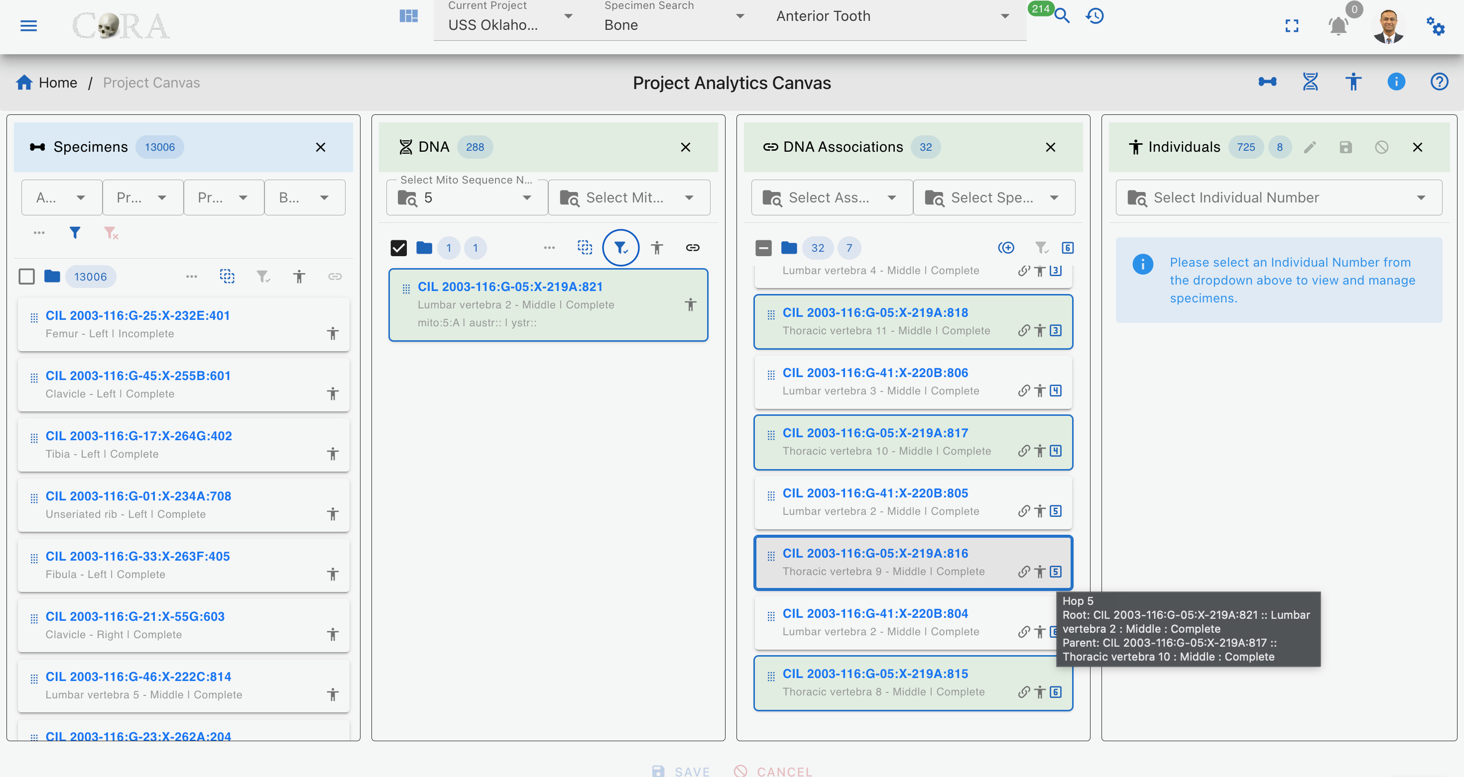
Association Type Filter
The DNA Association Lab table provides a filter for the 4 main specimen association types or relationships as shown below
| Association Type | Description |
|---|---|
| Articulations | Shows only Articulation specimen |
| Pair | Shows only paired specimens (e.g., left and right bones) |
| Refits | Shows only refitted fragments that rejoin to form a complete element |
| Morphology | Shows only morphological matches (similar morphological features) |
Associations List
Once filters are applied, the lab table displays the following information
- The key of each specimen type
- Underneath the specimen key Bone Name, Location and Status
- Right side of the specimen key Type of Relation, Human Icon
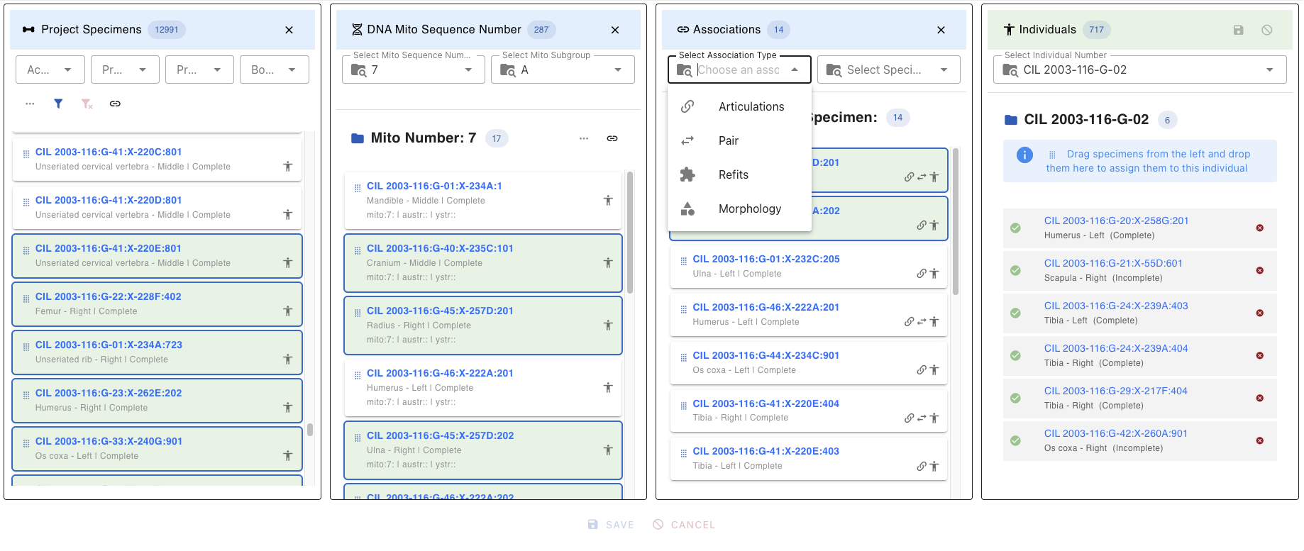
Associations Close/Hide
To close the Associations lab table lick the X button in the top-right corner of the lab table
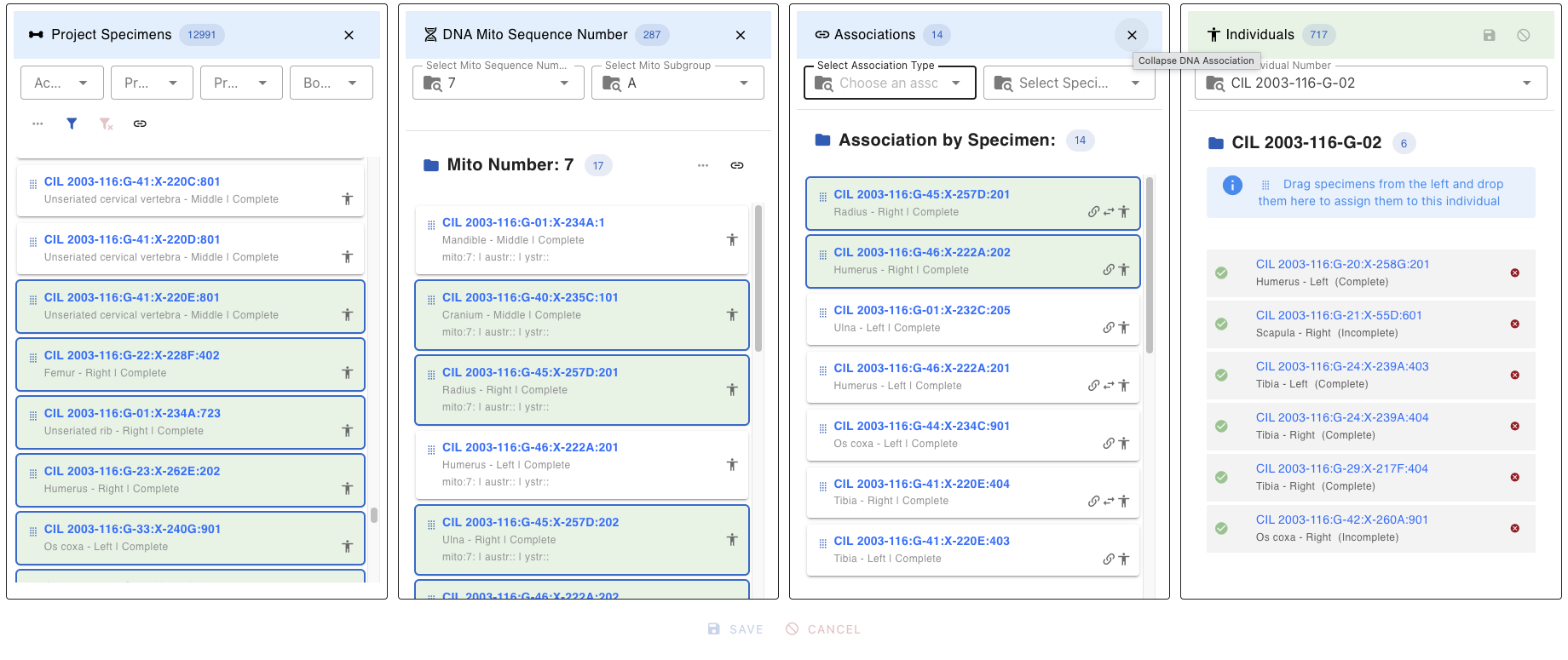
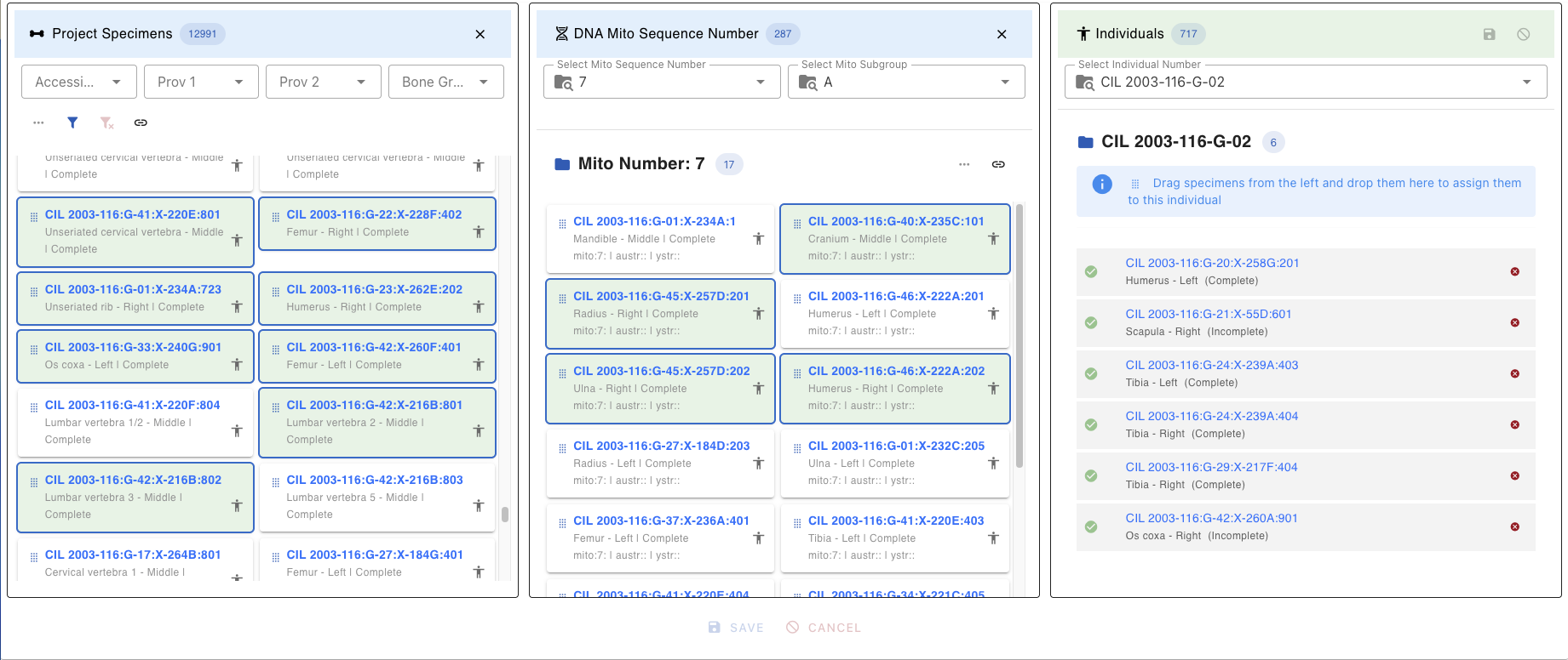
Individuals Lab Table
Displays a listing of all current individuals in the project and allows the user to select an individual to work including assignment of specimens to that individual. Once an individual number (identifier) is selected, all the pertinent information for that individual is displayed on the Individual Lab table.
Individual Selector
The dropdown at the top allows switching between individuals:
- Search by typing in the dropdown
- Select Individual Number
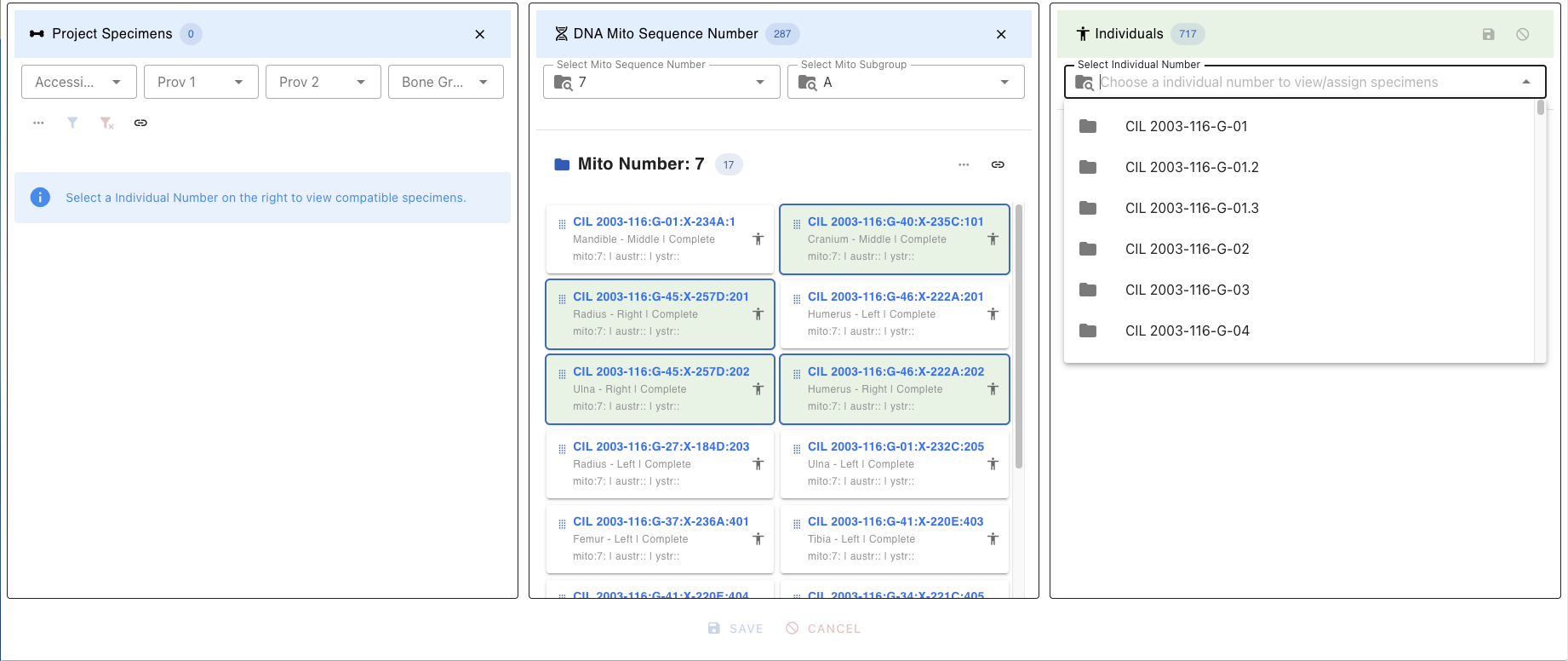
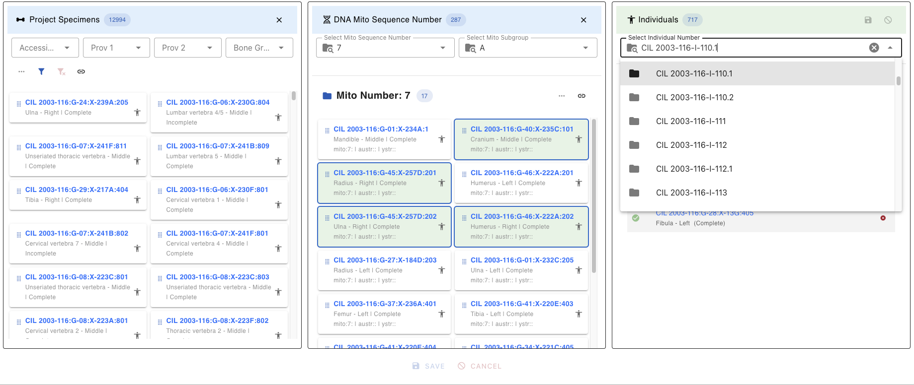
Individual Table Buttons/Icons
| Icon | Description |
|---|---|
| Enables editing of specimens under the selected individual. | |
| Saves all edits made to the individual and associated specimens. | |
| Cancels the current editing session without saving changes. | |
| Closes the individual lab table. | |
| Signifies the individual selected followed by the count of specimens on individual. | |
| Signifies the individual selected is locked for editing due to CHR Complete or Released | |
| Signifies the individual has DNA, followed by the actual DNA mito sequence number | |
| Signifies the individual has DNA with a subgroup such as A, B, or 1, 2.etc. | |
| Signifies the individual has Nuclear DNA, followed by the actual number | |
| Signifies the individual has Y-Str DNA, followed by the actual number | |
| Individual identification (ID )information such as remains status & dates | |
| Individual remains status (In Lab, In Analytics, CHR Complete, Released) | |
| Individual identification date if before Individual remains status | |
| Individual remains release date if after Individual remains status | |
| The red “X” icon marks the specimen for removal from the individual. | |
| Denotes articulation relationship, hovering over which displays the related articulated specimen | |
| Denotes pair match relationship, hovering over which displays the related pair match specimen | |
| Denotes refit relationship, hovering over which displays the related refit specimen | |
| Denotes morphology relationship, hovering over which displays the related morphology specimen |
Assigned Specimens
Displays all specimens currently assigned to the selected individual:
- Each specimen shows with a Green Checkmark (Complete)
- Can be removed by clicking the X from the right side of the card
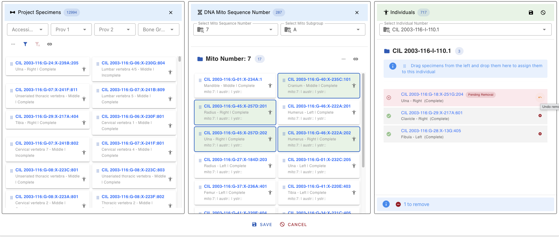
Assign Specimens to Individual
The Assign Specimen to Individual feature allows users to associate one or more specimens with a specific individual. This functionality is essential for grouping skeletal elements under a unique individual profile based on forensic analysis. Recent enhancements have introduced several new features to improve usability and functionality.
1. Select Individual
- Choose the target individual from the dropdown menu on the right panel.
- The selected individual’s details will be displayed.
2. Apply Filters (Optional)
Use the available filters shown below to refine the list of specimens displayed. You can use multiple filters for a more refined search.
- Accession
- Provenance 1
- Provenance 2
- Bone Group
- Bone
- Side
- Completeness
- Austr Sequence Number and Subgroup
- Ystr Sequence Number and Subgroup
3. Select DNA Mito # (Optional)
- Choose a DNA Mito Sequence Number from the dropdown menu to view and manage specimens associated with that sequence.
- Additional options include filtering by Mito Subgroup, Austr Sequence Number, and Ystr Sequence Number.
4. Select Association Type (Optional)
- Use the dropdown menu to select an association type (e.g., Articulations, Pair Match, Refits, Morphology).
- You can also select a specific specimen to view all associated specimens for the chosen association type.
5. Drag and Drop Specimens
- Select the desired specimens from the list on the left panel.
- Drag and drop the specimens into the individual’s assignment area on the right panel.
- Specimens marked for assignment or removal are visually distinguished with color-coded chips (e.g., orange for pending addition, red for pending removal).
6. Select Association Reasons
- For each specimen, select one or more reason for the association of that specimen to the individual from the dropdown menu. The table below shows all the association inclusion reasons and exclusion reasons
| Reasons | Icon | Inclusion | Exclusion |
|---|---|---|---|
| Mitochondrial DNA | |||
| Pair Match | |||
| Articulations | |||
| Accession | |||
| Anomaly | |||
| Chest Radiographic Comparison | |||
| Development | |||
| Isotope Analysis Report | |||
| Morphology | |||
| Nuclear DNA | |||
| Odontology | |||
| Osteometric Sorting | |||
| Pathology | |||
| Provenance | |||
| Refits | |||
| Taphonomy | |||
| Trauma |
7. Save or Cancel:
- To save the assignments, click the Save button.
- To cancel the entire process, click the Cancel button.
- You can also remove individual specimens from the assignment area by clicking the X icon next to them.
Key Features
- Dynamic Specimen List: The list updates based on applied filters, ensuring you only see relevant specimens.
- DNA Mito Sequence Integration: Manage specimens associated with specific DNA Mito Sequence Numbers.
- Association Management: View and manage specimens based on association types such as Articulations, Pairs, Refits, and Morphology.
- Reason Selection: Ensure each assignment has a documented reason for traceability.
- Bulk Assignment: Assign multiple specimens to an individual in one action using drag-and-drop functionality.
- Real-Time Updates: Changes are reflected immediately in the project database after saving.
- Action Alerts: Alerts at the bottom of the interface track pending assignments and removals.
Example Workflow
- Select an individual from the dropdown menu.
- Filter specimens by "Accession" and "Bone Group" or apply advanced filters like Austr Sequence Number or Ystr Subgroup.
- Select a DNA Mito Sequence Number to view related specimens.
- Choose an association type (e.g., Articulations) and select a specimen to view associated specimens.
- Drag and drop the filtered specimens into the individual’s assignment area.
- Click Save to save assignments.
- Select a reason for each assignment from the dropdown menu.
- Then click Save again to finalize the assignments.
Selection and Drag-and-Drop
Selecting Multiple Specimens
Single Selection:
- Click on a specimen card to select it
- Selected cards are highlighted with a green background color
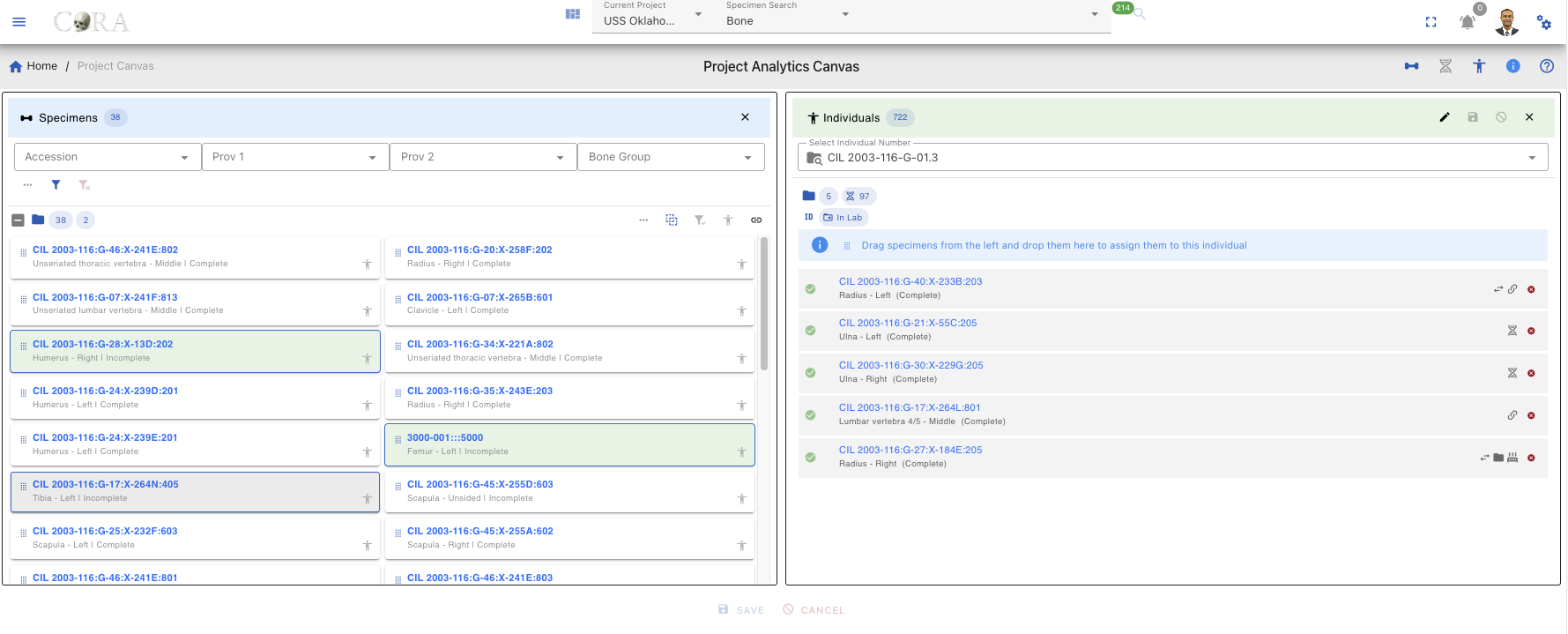
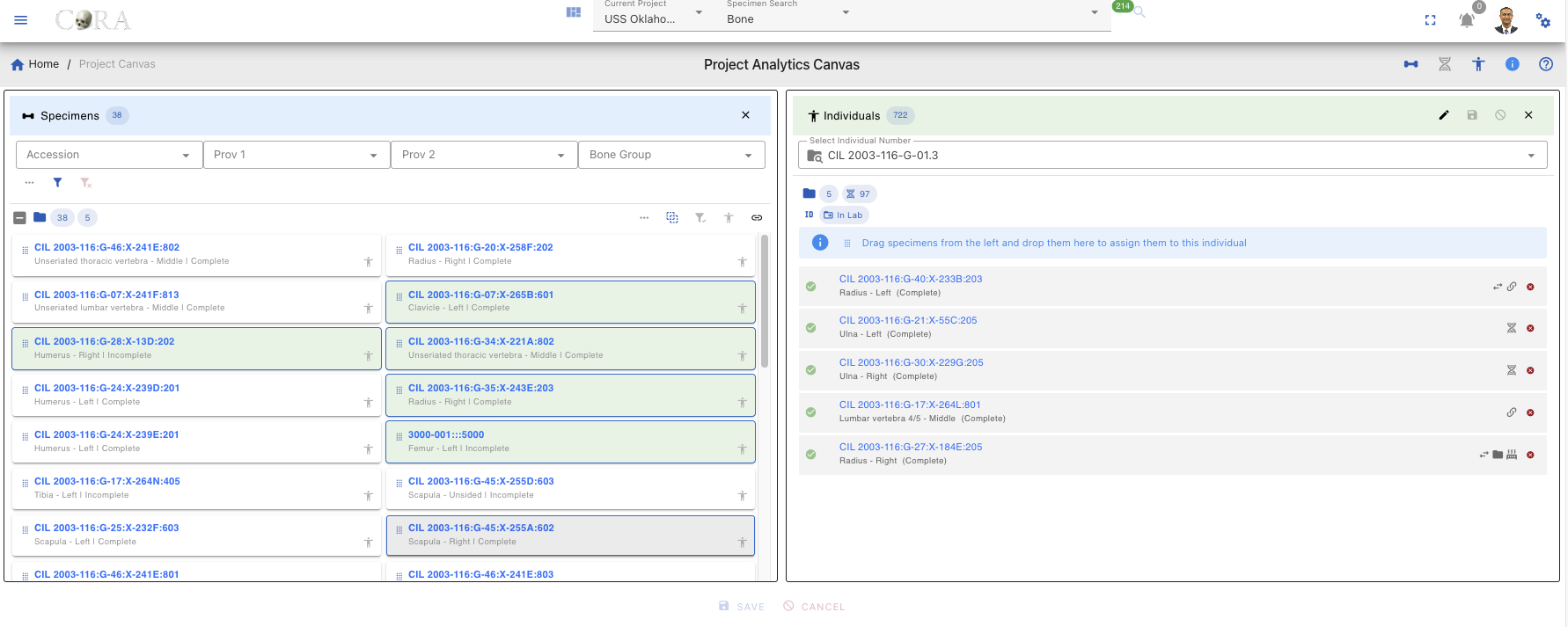
Multiple Selection:
| Method | Action |
|---|---|
| Ctrl/Cmd + Click | Add/remove individual specimens from selection |
| Shift + Click | Select range of specimens |
| Click + Drag | Draw selection box around multiple specimens |
| Ctrl/Cmd + A | Select all visible specimens |
Drag-and-Drop Assignment
To assign specimens to an individual:
- Ensure an individual is selected in the Individual Lab table
- Select one or more specimens in the Project Specimens or DNA Lab tables
- Click and hold on any selected specimen
- Drag toward the Individual Lab table
- Drop when the Individual Lab table highlights/accepts the drop
- Specimens appear in the Individual Lab table with "Pending Add" status (orange clock icon)
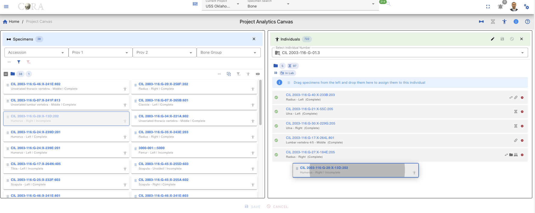
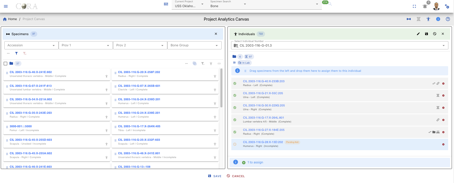
During Drag:
- Valid drop zone highlights in green color when dragging over it
- Invalid drops (e.g., no individual selected) show a rejection indicator
- Can drag multiple items at once
Remove Pending Assignments
Before saving, you can remove pending assignments by using the steps below
- Find the specimen in the Individual Lab table
- Click the X icon on the right side of the appropriate card
- Specimen turns in red color, and it reads as "Pending Removal"
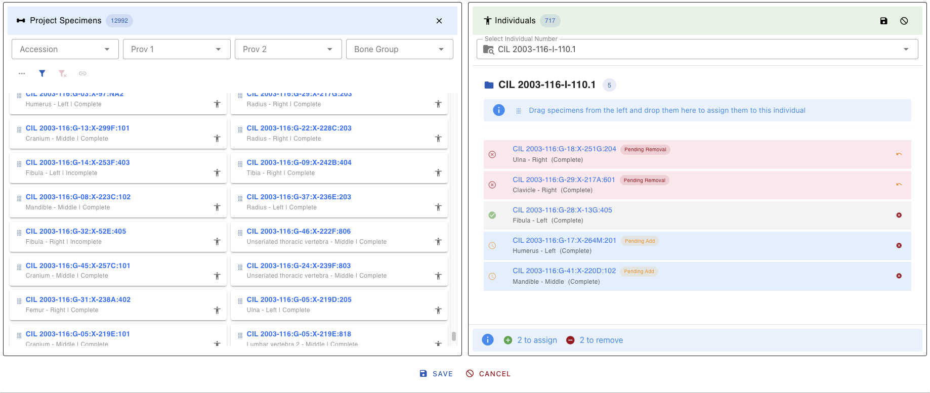
Saving Assignments
- Click the Save button in the Individual Lab table header
- Confirmation dialog opens titled "Confirm Specimen Assignments"
- Select a reason for each pending specimen from the dropdown:
- The Save button in the dialog is disabled until all pending items have a reason assigned
- Once all reasons are selected, click Save to complete the assignment
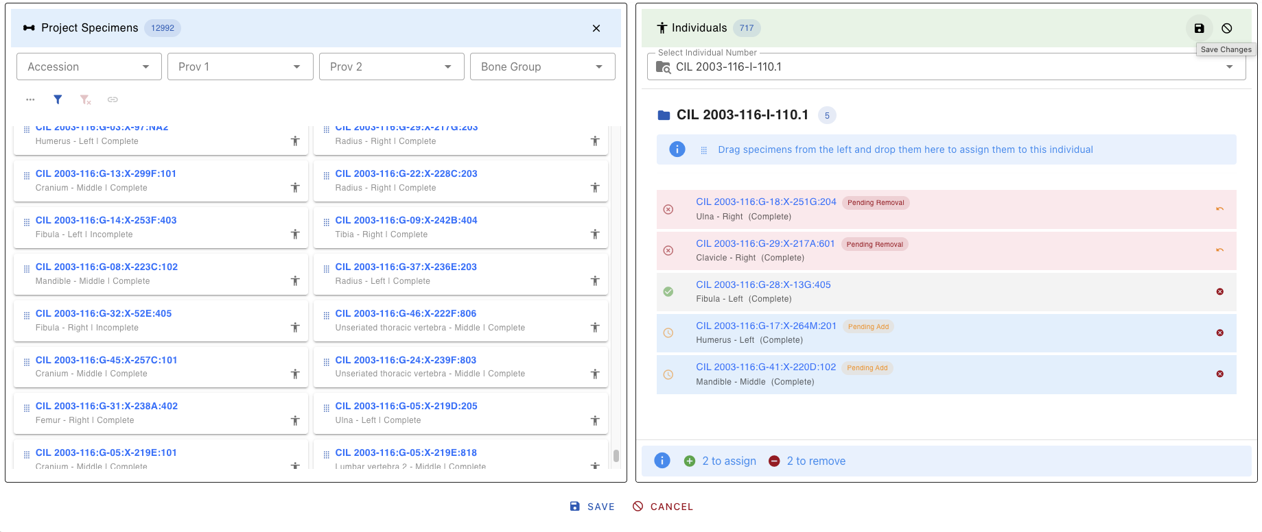

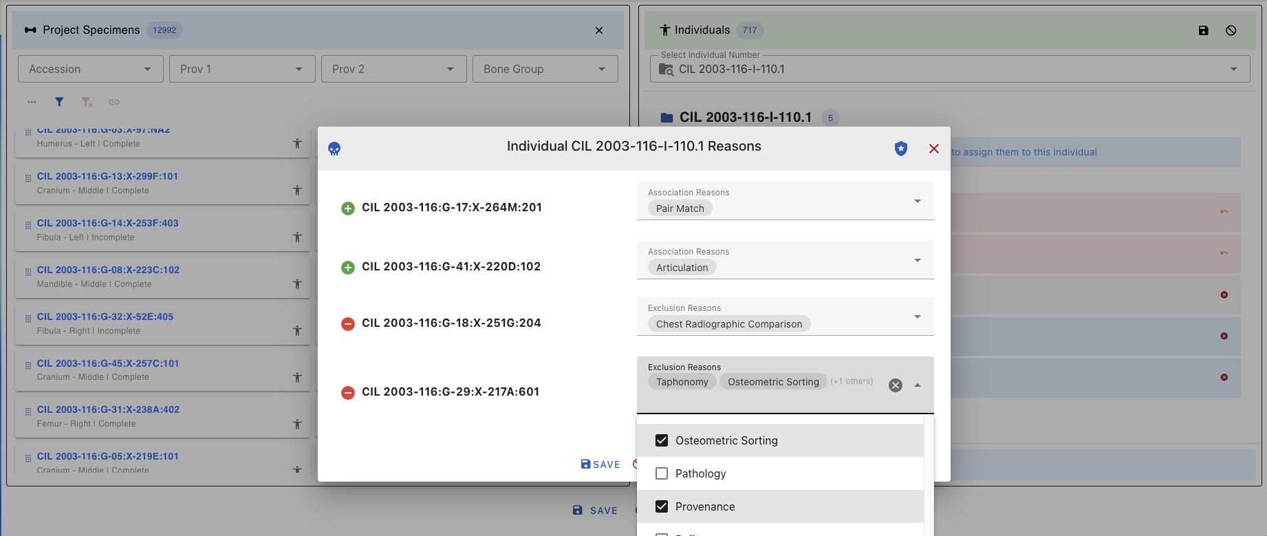
After Saving:
- Success notification appears
- Pending status changes to confirmed (human icon turns dark grey)
- Audit trail records the change with timestamp and user
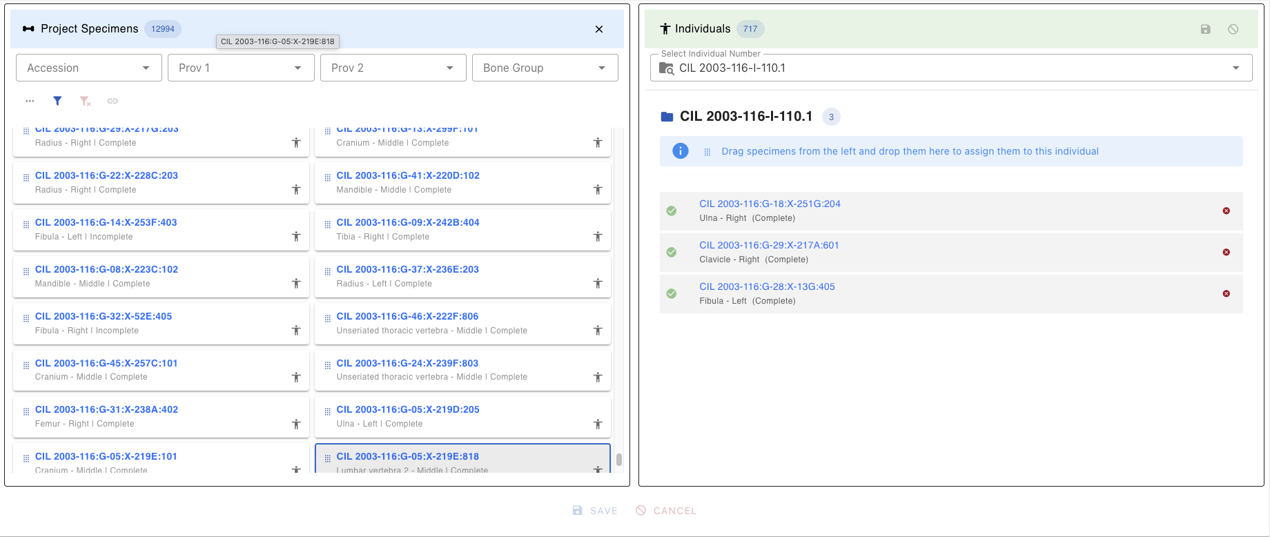
To discard changes:
- Click Cancel in the confirmation dialog, OR
- Refresh the page before saving
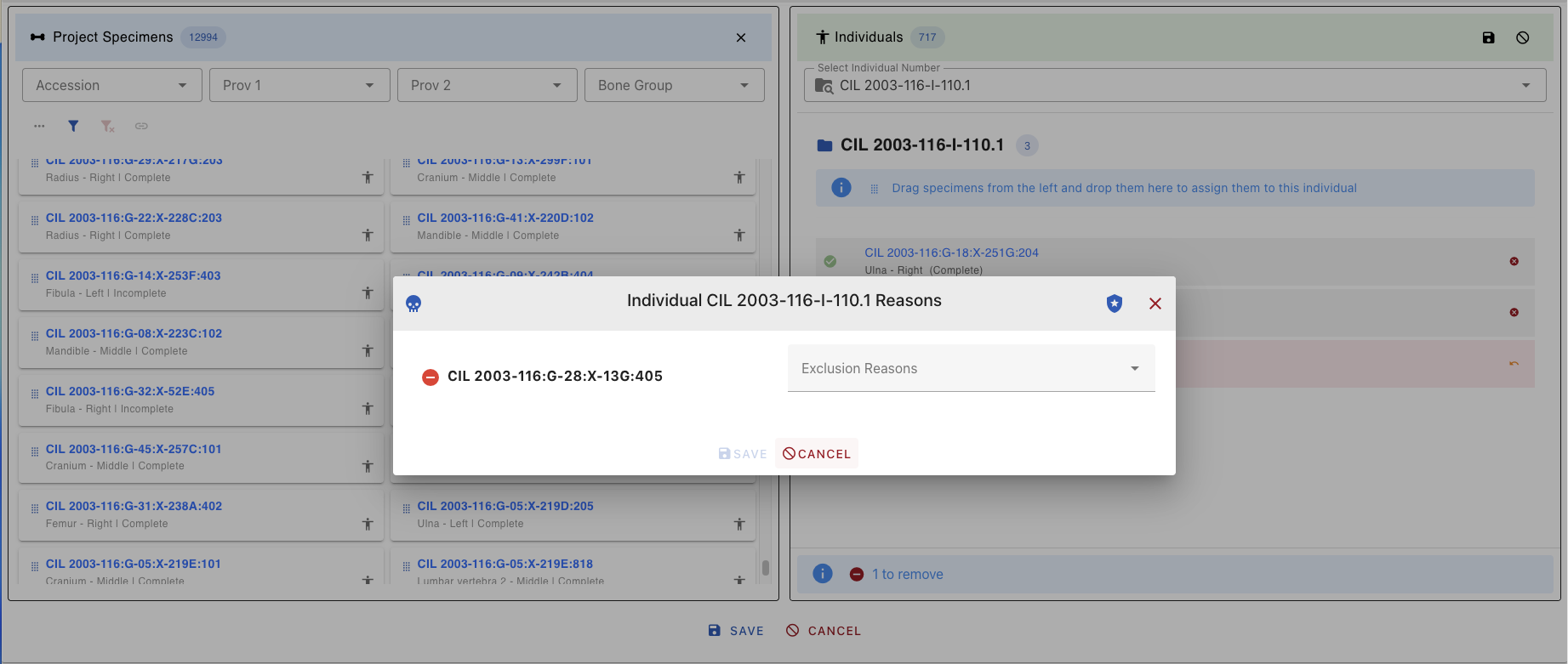
Quick Reference Tips
Filter and Search
- Use filters first to narrow large datasets before selecting specimens
- Combine filters within and across Lab tables for precise targeting of specimens
Icons and Status
- Dark Grey Human: Already assigned - be careful!
- Light Grey Human: Available for assignment
- Link Icon: Shows existing specimen connections
Assignment Process
- Select specimens → 2. Drag to Individual → 3. Add reasons → 4. Save
Common Issues
| Issue | Solution |
|---|---|
| Can't drop specimen | Ensure an individual is selected |
| Save button disabled | Assign reasons to all pending items |
| Can't see associations | Use the Link Button after selecting specimens |
Keyboard Shortcuts
| Shortcut | Action |
|---|---|
| Ctrl/Cmd + Click | Multi-select specimens |
| Shift + Click | Select range |
| Delete/Backspace | Remove selected from assignment |
| Ctrl/Cmd + S | Save (when in dialog) |
| Escape | Close dialog/cancel action |
Troubleshooting
Specimen Assignment Errors
Error Message:
"Cannot assign these specimens. The individual already has a complete specimen with the same bone and side, so only incomplete specimens are allowed."
Explanation:
This error occurs when you try to assign a complete specimen to an individual who already has a complete specimen of the same bone and side. In forensic anthropology, an individual can only have one complete specimen for each unique bone/side combination. However, incomplete specimens can still be assigned to complete the individual's skeletal representation.
Solution:
- Select incomplete specimens instead of complete ones when assigning to an individual who already has a complete specimen of the same bone and side
- Remove the existing complete specimen from the individual first (requires appropriate permissions), then assign the new complete specimen
- Use the filter to search for incomplete specimens by selecting "Incomplete" in the Completeness filter
Alternative Approaches:
- If you need to replace a complete specimen, first remove the existing complete specimen from the individual
- Consider if the specimen should be marked as "incomplete" if it's actually missing parts
- Contact your supervisor or system administrator if you believe the existing assignment is incorrect
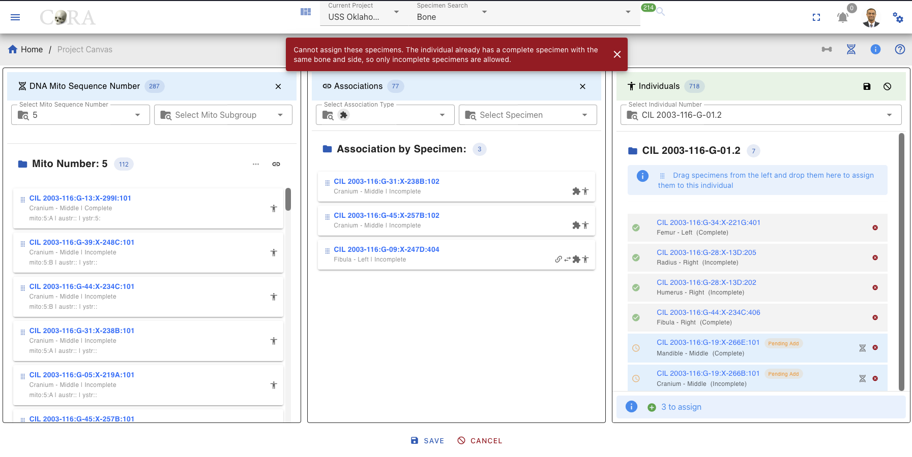
Reference
Country Language Timezone
Below you will find a listing of country, language and timezones settings supported in CoRA. You can use any of these to set the default country, default language and default timezones fields on the user model.
When a new user is created within an organization the default country, default language and default timezones are set to the organization's default country, default language and default timezones. Every user can change their individual setting in their My Profile page.
CoRA stores all date and time fields in UTC and then uses your default timezone settings to determine what timezone to use to display the date and time fields.
Country
| Code | Country | Flag |
|---|---|---|
| AF | Afghanistan |  |
| AX | Åland Islands |  |
| AL | Albania |  |
| DZ | Algeria |  |
| AS | American Samoa |  |
| AD | Andorra |  |
| AO | Angola |  |
| AI | Anguilla |  |
| AQ | Antarctica |  |
| AG | Antigua & Barbuda |  |
| AR | Argentina |  |
| AM | Armenia |  |
| AW | Aruba |  |
| AC | Ascension Island |  |
| AU | Australia |  |
| AT | Austria |  |
| AZ | Azerbaijan |  |
| BS | Bahamas |  |
| BH | Bahrain |  |
| BD | Bangladesh |  |
| BB | Barbados |  |
| BY | Belarus |  |
| BE | Belgium |  |
| BZ | Belize |  |
| BJ | Benin |  |
| BM | Bermuda |  |
| BT | Bhutan |  |
| BO | Bolivia |  |
| BA | Bosnia & Herzegovina |  |
| BW | Botswana |  |
| BR | Brazil |  |
| IO | British Indian Ocean Territory |  |
| VG | British Virgin Islands |  |
| BN | Brunei |  |
| BG | Bulgaria |  |
| BF | Burkina Faso |  |
| BI | Burundi |  |
| KH | Cambodia |  |
| CM | Cameroon |  |
| CA | Canada |  |
| IC | Canary Islands |  |
| CV | Cape Verde |  |
| BQ | Caribbean Netherlands |  |
| KY | Cayman Islands |  |
| CF | Central African Republic |  |
| EA | Ceuta & Melilla |  |
| TD | Chad |  |
| CL | Chile |  |
| CN | China |  |
| CX | Christmas Island |  |
| CC | Cocos (Keeling) Islands |  |
| CO | Colombia |  |
| KM | Comoros |  |
| CG | Congo - Brazzaville |  |
| CD | Congo - Kinshasa |  |
| CK | Cook Islands |  |
| CR | Costa Rica |  |
| CI | Côte d’Ivoire |  |
| HR | Croatia |  |
| CU | Cuba |  |
| CW | Curaçao |  |
| CY | Cyprus |  |
| CZ | Czechia |  |
| DK | Denmark |  |
| DG | Diego Garcia |  |
| DJ | Djibouti |  |
| DM | Dominica |  |
| DO | Dominican Republic |  |
| EC | Ecuador |  |
| EG | Egypt |  |
| SV | El Salvador |  |
| GQ | Equatorial Guinea |  |
| ER | Eritrea |  |
| EE | Estonia |  |
| ET | Ethiopia |  |
| EZ | Eurozone |  |
| FK | Falkland Islands |  |
| FO | Faroe Islands |  |
| FJ | Fiji |  |
| FI | Finland |  |
| FR | France |  |
| GF | French Guiana |  |
| PF | French Polynesia |  |
| TF | French Southern Territories |  |
| GA | Gabon |  |
| GM | Gambia |  |
| GE | Georgia |  |
| DE | Germany |  |
| GH | Ghana |  |
| GI | Gibraltar |  |
| GR | Greece |  |
| GL | Greenland |  |
| GD | Grenada |  |
| GP | Guadeloupe |  |
| GU | Guam |  |
| GT | Guatemala |  |
| GG | Guernsey |  |
| GN | Guinea |  |
| GW | Guinea-Bissau |  |
| GY | Guyana |  |
| HT | Haiti |  |
| HN | Honduras |  |
| HK | Hong Kong SAR China |  |
| HU | Hungary |  |
| IS | Iceland |  |
| IN | India |  |
| ID | Indonesia |  |
| IR | Iran |  |
| IQ | Iraq |  |
| IE | Ireland |  |
| IM | Isle of Man |  |
| IL | Israel |  |
| IT | Italy |  |
| JM | Jamaica |  |
| JP | Japan |  |
| JE | Jersey |  |
| JO | Jordan |  |
| KZ | Kazakhstan |  |
| KE | Kenya |  |
| KI | Kiribati |  |
| XK | Kosovo |  |
| KW | Kuwait |  |
| KG | Kyrgyzstan |  |
| LA | Laos |  |
| LV | Latvia |  |
| LB | Lebanon |  |
| LS | Lesotho |  |
| LR | Liberia |  |
| LY | Libya |  |
| LI | Liechtenstein |  |
| LT | Lithuania |  |
| LU | Luxembourg |  |
| MO | Macau SAR China |  |
| MK | Macedonia |  |
| MG | Madagascar |  |
| MW | Malawi |  |
| MY | Malaysia |  |
| MV | Maldives |  |
| ML | Mali |  |
| MT | Malta |  |
| MH | Marshall Islands |  |
| MQ | Martinique |  |
| MR | Mauritania |  |
| MU | Mauritius |  |
| YT | Mayotte |  |
| MX | Mexico |  |
| FM | Micronesia |  |
| MD | Moldova |  |
| MC | Monaco |  |
| MN | Mongolia |  |
| ME | Montenegro |  |
| MS | Montserrat |  |
| MA | Morocco |  |
| MZ | Mozambique |  |
| MM | Myanmar (Burma) |  |
| NA | Namibia |  |
| NR | Nauru |  |
| NP | Nepal |  |
| NL | Netherlands |  |
| NC | New Caledonia |  |
| NZ | New Zealand |  |
| NI | Nicaragua |  |
| NE | Niger |  |
| NG | Nigeria |  |
| NU | Niue |  |
| NF | Norfolk Island |  |
| KP | North Korea |  |
| MP | Northern Mariana Islands |  |
| NO | Norway |  |
| OM | Oman |  |
| PK | Pakistan |  |
| PW | Palau |  |
| PS | Palestinian Territories |  |
| PA | Panama |  |
| PG | Papua New Guinea |  |
| PY | Paraguay |  |
| PE | Peru |  |
| PH | Philippines |  |
| PN | Pitcairn Islands |  |
| PL | Poland |  |
| PT | Portugal |  |
| PR | Puerto Rico |  |
| QA | Qatar |  |
| RE | Réunion |  |
| RO | Romania |  |
| RU | Russia |  |
| RW | Rwanda |  |
| WS | Samoa |  |
| SM | San Marino |  |
| ST | São Tomé & Príncipe |  |
| SA | Saudi Arabia |  |
| SN | Senegal |  |
| RS | Serbia |  |
| SC | Seychelles |  |
| SL | Sierra Leone |  |
| SG | Singapore |  |
| SX | Sint Maarten |  |
| SK | Slovakia |  |
| SI | Slovenia |  |
| SB | Solomon Islands |  |
| SO | Somalia |  |
| ZA | South Africa |  |
| GS | South Georgia & South Sandwich Islands |  |
| KR | South Korea |  |
| SS | South Sudan |  |
| ES | Spain |  |
| LK | Sri Lanka |  |
| BL | St. Barthélemy |  |
| SH | St. Helena |  |
| KN | St. Kitts & Nevis |  |
| LC | St. Lucia |  |
| MF | St. Martin |  |
| PM | St. Pierre & Miquelon |  |
| VC | St. Vincent & Grenadines |  |
| SD | Sudan |  |
| SR | Suriname |  |
| SJ | Svalbard & Jan Mayen |  |
| SZ | Swaziland |  |
| SE | Sweden |  |
| CH | Switzerland |  |
| SY | Syria |  |
| TW | Taiwan |  |
| TJ | Tajikistan |  |
| TZ | Tanzania |  |
| TH | Thailand |  |
| TL | Timor-Leste |  |
| TG | Togo |  |
| TK | Tokelau |  |
| TO | Tonga |  |
| TT | Trinidad & Tobago |  |
| TA | Tristan da Cunha |  |
| TN | Tunisia |  |
| TR | Turkey |  |
| TM | Turkmenistan |  |
| TC | Turks & Caicos Islands |  |
| TV | Tuvalu |  |
| UM | U.S. Outlying Islands |  |
| VI | U.S. Virgin Islands |  |
| UG | Uganda |  |
| UA | Ukraine |  |
| AE | United Arab Emirates |  |
| GB | United Kingdom | |
| UN | United Nations | :un: |
| US | United States |  |
| UY | Uruguay |  |
| UZ | Uzbekistan |  |
| VU | Vanuatu |  |
| VA | Vatican City |  |
| VE | Venezuela |  |
| VN | Vietnam |  |
| WF | Wallis & Futuna |  |
| EH | Western Sahara |  |
| YE | Yemen |  |
| ZM | Zambia |  |
| ZW | Zimbabwe |  |
Language
| Code | Country |
|---|---|
| en | English |
| aa | Afar |
| ab | Abkhazian |
| af | Afrikaans |
| am | Amharic |
| ar | Arabic |
| as | Assamese |
| ay | Aymara |
| az | Azerbaijani |
| ba | Bashkir |
| be | Byelorussian |
| bg | Bulgarian |
| bh | Bihari |
| bi | Bislama |
| bn | Bengali/Bangla |
| bo | Tibetan |
| br | Breton |
| ca | Catalan |
| co | Corsican |
| cs | Czech |
| cy | Welsh |
| da | Danish |
| de | German |
| dz | Bhutani |
| el | Greek |
| eo | Esperanto |
| es | Spanish |
| et | Estonian |
| eu | Basque |
| fa | Persian |
| fi | Finnish |
| fj | Fiji |
| fo | Faeroese |
| fr | French |
| fy | Frisian |
| ga | Irish |
| gd | Scots/Gaelic |
| gl | Galician |
| gn | Guarani |
| gu | Gujarati |
| ha | Hausa |
| hi | Hindi |
| hr | Croatian |
| hu | Hungarian |
| hy | Armenian |
| ia | Interlingua |
| ie | Interlingue |
| ik | Inupiak |
| in | Indonesian |
| is | Icelandic |
| it | Italian |
| iw | Hebrew |
| ja | Japanese |
| ji | Yiddish |
| jw | Javanese |
| ka | Georgian |
| kk | Kazakh |
| kl | Greenlandic |
| km | Cambodian |
| kn | Kannada |
| ko | Korean |
| ks | Kashmiri |
| ku | Kurdish |
| ky | Kirghiz |
| la | Latin |
| ln | Lingala |
| lo | Laothian |
| lt | Lithuanian |
| lv | Latvian/Lettish |
| mg | Malagasy |
| mi | Maori |
| mk | Macedonian |
| ml | Malayalam |
| mn | Mongolian |
| mo | Moldavian |
| mr | Marathi |
| ms | Malay |
| mt | Maltese |
| my | Burmese |
| na | Nauru |
| ne | Nepali |
| nl | Dutch |
| no | Norwegian |
| oc | Occitan |
| om | (Afan)/Oromoor/Oriya |
| pa | Punjabi |
| pl | Polish |
| ps | Pashto/Pushto |
| pt | Portuguese |
| qu | Quechua |
| rm | Rhaeto-Romance |
| rn | Kirundi |
| ro | Romanian |
| ru | Russian |
| rw | Kinyarwanda |
| sa | Sanskrit |
| sd | Sindhi |
| sg | Sangro |
| sh | Serbo-Croatian |
| si | Singhalese |
| sk | Slovak |
| sl | Slovenian |
| sm | Samoan |
| sn | Shona |
| so | Somali |
| sq | Albanian |
| sr | Serbian |
| ss | Siswati |
| st | Sesotho |
| su | Sundanese |
| sv | Swedish |
| sw | Swahili |
| ta | Tamil |
| te | Tegulu |
| tg | Tajik |
| th | Thai |
| ti | Tigrinya |
| tk | Turkmen |
| tl | Tagalog |
| tn | Setswana |
| to | Tonga |
| tr | Turkish |
| ts | Tsonga |
| tt | Tatar |
| tw | Twi |
| uk | Ukrainian |
| ur | Urdu |
| uz | Uzbek |
| vi | Vietnamese |
| vo | Volapuk |
| wo | Wolof |
| xh | Xhosa |
| yo | Yoruba |
| zh | Chinese |
| zu | Zulu |
Timezone
| Code | Country |
|---|---|
| Pacific/Midway | (UTC-11:00) Midway |
| Pacific/Niue | (UTC-11:00) Niue |
| Pacific/Pago_Pago | (UTC-11:00) Pago Pago |
| America/Adak | (UTC-10:00) Adak |
| Pacific/Honolulu | (UTC-10:00) Honolulu |
| Pacific/Johnston | (UTC-10:00) Johnston |
| Pacific/Rarotonga | (UTC-10:00) Rarotonga |
| Pacific/Tahiti | (UTC-10:00) Tahiti |
| Pacific/Marquesas | (UTC-09:30) Marquesas |
| America/Anchorage | (UTC-09:00) Anchorage |
| Pacific/Gambier | (UTC-09:00) Gambier |
| America/Juneau | (UTC-09:00) Juneau |
| America/Nome | (UTC-09:00) Nome |
| America/Sitka | (UTC-09:00) Sitka |
| America/Yakutat | (UTC-09:00) Yakutat |
| America/Dawson | (UTC-08:00) Dawson |
| America/Los_Angeles | (UTC-08:00) Los Angeles |
| America/Metlakatla | (UTC-08:00) Metlakatla |
| Pacific/Pitcairn | (UTC-08:00) Pitcairn |
| America/Santa_Isabel | (UTC-08:00) Santa Isabel |
| America/Tijuana | (UTC-08:00) Tijuana |
| America/Vancouver | (UTC-08:00) Vancouver |
| America/Whitehorse | (UTC-08:00) Whitehorse |
| America/Boise | (UTC-07:00) Boise |
| America/Cambridge_Bay | (UTC-07:00) Cambridge Bay |
| America/Chihuahua | (UTC-07:00) Chihuahua |
| America/Creston | (UTC-07:00) Creston |
| America/Dawson_Creek | (UTC-07:00) Dawson Creek |
| America/Denver | (UTC-07:00) Denver |
| America/Edmonton | (UTC-07:00) Edmonton |
| America/Hermosillo | (UTC-07:00) Hermosillo |
| America/Inuvik | (UTC-07:00) Inuvik |
| America/Mazatlan | (UTC-07:00) Mazatlan |
| America/Ojinaga | (UTC-07:00) Ojinaga |
| America/Phoenix | (UTC-07:00) Phoenix |
| America/Shiprock | (UTC-07:00) Shiprock |
| America/Yellowknife | (UTC-07:00) Yellowknife |
| America/Bahia_Banderas | (UTC-06:00) Bahia Banderas |
| America/Belize | (UTC-06:00) Belize |
| America/North_Dakota/Beulah | (UTC-06:00) Beulah |
| America/Cancun | (UTC-06:00) Cancun |
| America/North_Dakota/Center | (UTC-06:00) Center |
| America/Chicago | (UTC-06:00) Chicago |
| America/Costa_Rica | (UTC-06:00) Costa Rica |
| Pacific/Easter | (UTC-06:00) Easter |
| America/El_Salvador | (UTC-06:00) El Salvador |
| Pacific/Galapagos | (UTC-06:00) Galapagos |
| America/Guatemala | (UTC-06:00) Guatemala |
| America/Indiana/Knox | (UTC-06:00) Knox |
| America/Managua | (UTC-06:00) Managua |
| America/Matamoros | (UTC-06:00) Matamoros |
| America/Menominee | (UTC-06:00) Menominee |
| America/Merida | (UTC-06:00) Merida |
| America/Mexico_City | (UTC-06:00) Mexico City |
| America/Monterrey | (UTC-06:00) Monterrey |
| America/North_Dakota/New_Salem | (UTC-06:00) New Salem |
| America/Rainy_River | (UTC-06:00) Rainy River |
| America/Rankin_Inlet | (UTC-06:00) Rankin Inlet |
| America/Regina | (UTC-06:00) Regina |
| America/Resolute | (UTC-06:00) Resolute |
| America/Swift_Current | (UTC-06:00) Swift Current |
| America/Tegucigalpa | (UTC-06:00) Tegucigalpa |
| America/Indiana/Tell_City | (UTC-06:00) Tell City |
| America/Winnipeg | (UTC-06:00) Winnipeg |
| America/Atikokan | (UTC-05:00) Atikokan |
| America/Bogota | (UTC-05:00) Bogota |
| America/Cayman | (UTC-05:00) Cayman |
| America/Detroit | (UTC-05:00) Detroit |
| America/Grand_Turk | (UTC-05:00) Grand Turk |
| America/Guayaquil | (UTC-05:00) Guayaquil |
| America/Havana | (UTC-05:00) Havana |
| America/Indiana/Indianapolis | (UTC-05:00) Indianapolis |
| America/Iqaluit | (UTC-05:00) Iqaluit |
| America/Jamaica | (UTC-05:00) Jamaica |
| America/Lima | (UTC-05:00) Lima |
| America/Kentucky/Louisville | (UTC-05:00) Louisville |
| America/Indiana/Marengo | (UTC-05:00) Marengo |
| America/Kentucky/Monticello | (UTC-05:00) Monticello |
| America/Montreal | (UTC-05:00) Montreal |
| America/Nassau | (UTC-05:00) Nassau |
| America/New_York | (UTC-05:00) New York |
| America/Nipigon | (UTC-05:00) Nipigon |
| America/Panama | (UTC-05:00) Panama |
| America/Pangnirtung | (UTC-05:00) Pangnirtung |
| America/Indiana/Petersburg | (UTC-05:00) Petersburg |
| America/Port-au-Prince | (UTC-05:00) Port-au-Prince |
| America/Thunder_Bay | (UTC-05:00) Thunder Bay |
| America/Toronto | (UTC-05:00) Toronto |
| America/Indiana/Vevay | (UTC-05:00) Vevay |
| America/Indiana/Vincennes | (UTC-05:00) Vincennes |
| America/Indiana/Winamac | (UTC-05:00) Winamac |
| America/Caracas | (UTC-04:30) Caracas |
| America/Anguilla | (UTC-04:00) Anguilla |
| America/Antigua | (UTC-04:00) Antigua |
| America/Aruba | (UTC-04:00) Aruba |
| America/Asuncion | (UTC-04:00) Asuncion |
| America/Barbados | (UTC-04:00) Barbados |
| Atlantic/Bermuda | (UTC-04:00) Bermuda |
| America/Blanc-Sablon | (UTC-04:00) Blanc-Sablon |
| America/Boa_Vista | (UTC-04:00) Boa Vista |
| America/Campo_Grande | (UTC-04:00) Campo Grande |
| America/Cuiaba | (UTC-04:00) Cuiaba |
| America/Curacao | (UTC-04:00) Curacao |
| America/Dominica | (UTC-04:00) Dominica |
| America/Eirunepe | (UTC-04:00) Eirunepe |
| America/Glace_Bay | (UTC-04:00) Glace Bay |
| America/Goose_Bay | (UTC-04:00) Goose Bay |
| America/Grenada | (UTC-04:00) Grenada |
| America/Guadeloupe | (UTC-04:00) Guadeloupe |
| America/Guyana | (UTC-04:00) Guyana |
| America/Halifax | (UTC-04:00) Halifax |
| America/Kralendijk | (UTC-04:00) Kralendijk |
| America/La_Paz | (UTC-04:00) La Paz |
| America/Lower_Princes | (UTC-04:00) Lower Princes |
| America/Manaus | (UTC-04:00) Manaus |
| America/Marigot | (UTC-04:00) Marigot |
| America/Martinique | (UTC-04:00) Martinique |
| America/Moncton | (UTC-04:00) Moncton |
| America/Montserrat | (UTC-04:00) Montserrat |
| Antarctica/Palmer | (UTC-04:00) Palmer |
| America/Port_of_Spain | (UTC-04:00) Port of Spain |
| America/Porto_Velho | (UTC-04:00) Porto Velho |
| America/Puerto_Rico | (UTC-04:00) Puerto Rico |
| America/Rio_Branco | (UTC-04:00) Rio Branco |
| America/Santiago | (UTC-04:00) Santiago |
| America/Santo_Domingo | (UTC-04:00) Santo Domingo |
| America/St_Barthelemy | (UTC-04:00) St. Barthelemy |
| America/St_Kitts | (UTC-04:00) St. Kitts |
| America/St_Lucia | (UTC-04:00) St. Lucia |
| America/St_Thomas | (UTC-04:00) St. Thomas |
| America/St_Vincent | (UTC-04:00) St. Vincent |
| America/Thule | (UTC-04:00) Thule |
| America/Tortola | (UTC-04:00) Tortola |
| America/St_Johns | (UTC-03:30) St. Johns |
| America/Araguaina | (UTC-03:00) Araguaina |
| America/Bahia | (UTC-03:00) Bahia |
| America/Belem | (UTC-03:00) Belem |
| America/Argentina/Buenos_Aires | (UTC-03:00) Buenos Aires |
| America/Argentina/Catamarca | (UTC-03:00) Catamarca |
| America/Cayenne | (UTC-03:00) Cayenne |
| America/Argentina/Cordoba | (UTC-03:00) Cordoba |
| America/Fortaleza | (UTC-03:00) Fortaleza |
| America/Godthab | (UTC-03:00) Godthab |
| America/Argentina/Jujuy | (UTC-03:00) Jujuy |
| America/Argentina/La_Rioja | (UTC-03:00) La Rioja |
| America/Maceio | (UTC-03:00) Maceio |
| America/Argentina/Mendoza | (UTC-03:00) Mendoza |
| America/Miquelon | (UTC-03:00) Miquelon |
| America/Montevideo | (UTC-03:00) Montevideo |
| America/Paramaribo | (UTC-03:00) Paramaribo |
| America/Recife | (UTC-03:00) Recife |
| America/Argentina/Rio_Gallegos | (UTC-03:00) Rio Gallegos |
| Antarctica/Rothera | (UTC-03:00) Rothera |
| America/Argentina/Salta | (UTC-03:00) Salta |
| America/Argentina/San_Juan | (UTC-03:00) San Juan |
| America/Argentina/San_Luis | (UTC-03:00) San Luis |
| America/Santarem | (UTC-03:00) Santarem |
| America/Sao_Paulo | (UTC-03:00) Sao Paulo |
| Atlantic/Stanley | (UTC-03:00) Stanley |
| America/Argentina/Tucuman | (UTC-03:00) Tucuman |
| America/Argentina/Ushuaia | (UTC-03:00) Ushuaia |
| America/Noronha | (UTC-02:00) Noronha |
| Atlantic/South_Georgia | (UTC-02:00) South Georgia |
| Atlantic/Azores | (UTC-01:00) Azores |
| Atlantic/Cape_Verde | (UTC-01:00) Cape Verde |
| America/Scoresbysund | (UTC-01:00) Scoresbysund |
| Africa/Abidjan | (UTC+00:00) Abidjan |
| Africa/Accra | (UTC+00:00) Accra |
| Africa/Bamako | (UTC+00:00) Bamako |
| Africa/Banjul | (UTC+00:00) Banjul |
| Africa/Bissau | (UTC+00:00) Bissau |
| Atlantic/Canary | (UTC+00:00) Canary |
| Africa/Casablanca | (UTC+00:00) Casablanca |
| Africa/Conakry | (UTC+00:00) Conakry |
| Africa/Dakar | (UTC+00:00) Dakar |
| America/Danmarkshavn | (UTC+00:00) Danmarkshavn |
| Europe/Dublin | (UTC+00:00) Dublin |
| Africa/El_Aaiun | (UTC+00:00) El Aaiun |
| Atlantic/Faroe | (UTC+00:00) Faroe |
| Africa/Freetown | (UTC+00:00) Freetown |
| Europe/Guernsey | (UTC+00:00) Guernsey |
| Europe/Isle_of_Man | (UTC+00:00) Isle of Man |
| Europe/Jersey | (UTC+00:00) Jersey |
| Europe/Lisbon | (UTC+00:00) Lisbon |
| Africa/Lome | (UTC+00:00) Lome |
| Europe/London | (UTC+00:00) London |
| Atlantic/Madeira | (UTC+00:00) Madeira |
| Africa/Monrovia | (UTC+00:00) Monrovia |
| Africa/Nouakchott | (UTC+00:00) Nouakchott |
| Africa/Ouagadougou | (UTC+00:00) Ouagadougou |
| Atlantic/Reykjavik | (UTC+00:00) Reykjavik |
| Africa/Sao_Tome | (UTC+00:00) Sao Tome |
| Atlantic/St_Helena | (UTC+00:00) St. Helena |
| UTC | (UTC+00:00) UTC |
| Africa/Algiers | (UTC+01:00) Algiers |
| Europe/Amsterdam | (UTC+01:00) Amsterdam |
| Europe/Andorra | (UTC+01:00) Andorra |
| Africa/Bangui | (UTC+01:00) Bangui |
| Europe/Belgrade | (UTC+01:00) Belgrade |
| Europe/Berlin | (UTC+01:00) Berlin |
| Europe/Bratislava | (UTC+01:00) Bratislava |
| Africa/Brazzaville | (UTC+01:00) Brazzaville |
| Europe/Brussels | (UTC+01:00) Brussels |
| Europe/Budapest | (UTC+01:00) Budapest |
| Europe/Busingen | (UTC+01:00) Busingen |
| Africa/Ceuta | (UTC+01:00) Ceuta |
| Europe/Copenhagen | (UTC+01:00) Copenhagen |
| Africa/Douala | (UTC+01:00) Douala |
| Europe/Gibraltar | (UTC+01:00) Gibraltar |
| Africa/Kinshasa | (UTC+01:00) Kinshasa |
| Africa/Lagos | (UTC+01:00) Lagos |
| Africa/Libreville | (UTC+01:00) Libreville |
| Europe/Ljubljana | (UTC+01:00) Ljubljana |
| Arctic/Longyearbyen | (UTC+01:00) Longyearbyen |
| Africa/Luanda | (UTC+01:00) Luanda |
| Europe/Luxembourg | (UTC+01:00) Luxembourg |
| Europe/Madrid | (UTC+01:00) Madrid |
| Africa/Malabo | (UTC+01:00) Malabo |
| Europe/Malta | (UTC+01:00) Malta |
| Europe/Monaco | (UTC+01:00) Monaco |
| Africa/Ndjamena | (UTC+01:00) Ndjamena |
| Africa/Niamey | (UTC+01:00) Niamey |
| Europe/Oslo | (UTC+01:00) Oslo |
| Europe/Paris | (UTC+01:00) Paris |
| Europe/Podgorica | (UTC+01:00) Podgorica |
| Africa/Porto-Novo | (UTC+01:00) Porto-Novo |
| Europe/Prague | (UTC+01:00) Prague |
| Europe/Rome | (UTC+01:00) Rome |
| Europe/San_Marino | (UTC+01:00) San Marino |
| Europe/Sarajevo | (UTC+01:00) Sarajevo |
| Europe/Skopje | (UTC+01:00) Skopje |
| Europe/Stockholm | (UTC+01:00) Stockholm |
| Europe/Tirane | (UTC+01:00) Tirane |
| Africa/Tripoli | (UTC+01:00) Tripoli |
| Africa/Tunis | (UTC+01:00) Tunis |
| Europe/Vaduz | (UTC+01:00) Vaduz |
| Europe/Vatican | (UTC+01:00) Vatican |
| Europe/Vienna | (UTC+01:00) Vienna |
| Europe/Warsaw | (UTC+01:00) Warsaw |
| Africa/Windhoek | (UTC+01:00) Windhoek |
| Europe/Zagreb | (UTC+01:00) Zagreb |
| Europe/Zurich | (UTC+01:00) Zurich |
| Europe/Athens | (UTC+02:00) Athens |
| Asia/Beirut | (UTC+02:00) Beirut |
| Africa/Blantyre | (UTC+02:00) Blantyre |
| Europe/Bucharest | (UTC+02:00) Bucharest |
| Africa/Bujumbura | (UTC+02:00) Bujumbura |
| Africa/Cairo | (UTC+02:00) Cairo |
| Europe/Chisinau | (UTC+02:00) Chisinau |
| Asia/Damascus | (UTC+02:00) Damascus |
| Africa/Gaborone | (UTC+02:00) Gaborone |
| Asia/Gaza | (UTC+02:00) Gaza |
| Africa/Harare | (UTC+02:00) Harare |
| Asia/Hebron | (UTC+02:00) Hebron |
| Europe/Helsinki | (UTC+02:00) Helsinki |
| Europe/Istanbul | (UTC+02:00) Istanbul |
| Asia/Jerusalem | (UTC+02:00) Jerusalem |
| Africa/Johannesburg | (UTC+02:00) Johannesburg |
| Europe/Kiev | (UTC+02:00) Kiev |
| Africa/Kigali | (UTC+02:00) Kigali |
| Africa/Lubumbashi | (UTC+02:00) Lubumbashi |
| Africa/Lusaka | (UTC+02:00) Lusaka |
| Africa/Maputo | (UTC+02:00) Maputo |
| Europe/Mariehamn | (UTC+02:00) Mariehamn |
| Africa/Maseru | (UTC+02:00) Maseru |
| Africa/Mbabane | (UTC+02:00) Mbabane |
| Asia/Nicosia | (UTC+02:00) Nicosia |
| Europe/Riga | (UTC+02:00) Riga |
| Europe/Simferopol | (UTC+02:00) Simferopol |
| Europe/Sofia | (UTC+02:00) Sofia |
| Europe/Tallinn | (UTC+02:00) Tallinn |
| Europe/Uzhgorod | (UTC+02:00) Uzhgorod |
| Europe/Vilnius | (UTC+02:00) Vilnius |
| Europe/Zaporozhye | (UTC+02:00) Zaporozhye |
| Africa/Addis_Ababa | (UTC+03:00) Addis Ababa |
| Asia/Aden | (UTC+03:00) Aden |
| Asia/Amman | (UTC+03:00) Amman |
| Indian/Antananarivo | (UTC+03:00) Antananarivo |
| Africa/Asmara | (UTC+03:00) Asmara |
| Asia/Baghdad | (UTC+03:00) Baghdad |
| Asia/Bahrain | (UTC+03:00) Bahrain |
| Indian/Comoro | (UTC+03:00) Comoro |
| Africa/Dar_es_Salaam | (UTC+03:00) Dar es Salaam |
| Africa/Djibouti | (UTC+03:00) Djibouti |
| Africa/Juba | (UTC+03:00) Juba |
| Europe/Kaliningrad | (UTC+03:00) Kaliningrad |
| Africa/Kampala | (UTC+03:00) Kampala |
| Africa/Khartoum | (UTC+03:00) Khartoum |
| Asia/Kuwait | (UTC+03:00) Kuwait |
| Indian/Mayotte | (UTC+03:00) Mayotte |
| Europe/Minsk | (UTC+03:00) Minsk |
| Africa/Mogadishu | (UTC+03:00) Mogadishu |
| Africa/Nairobi | (UTC+03:00) Nairobi |
| Asia/Qatar | (UTC+03:00) Qatar |
| Asia/Riyadh | (UTC+03:00) Riyadh |
| Antarctica/Syowa | (UTC+03:00) Syowa |
| Asia/Tehran | (UTC+03:30) Tehran |
| Asia/Baku | (UTC+04:00) Baku |
| Asia/Dubai | (UTC+04:00) Dubai |
| Indian/Mahe | (UTC+04:00) Mahe |
| Indian/Mauritius | (UTC+04:00) Mauritius |
| Europe/Moscow | (UTC+04:00) Moscow |
| Asia/Muscat | (UTC+04:00) Muscat |
| Indian/Reunion | (UTC+04:00) Reunion |
| Europe/Samara | (UTC+04:00) Samara |
| Asia/Tbilisi | (UTC+04:00) Tbilisi |
| Europe/Volgograd | (UTC+04:00) Volgograd |
| Asia/Yerevan | (UTC+04:00) Yerevan |
| Asia/Kabul | (UTC+04:30) Kabul |
| Asia/Aqtau | (UTC+05:00) Aqtau |
| Asia/Aqtobe | (UTC+05:00) Aqtobe |
| Asia/Ashgabat | (UTC+05:00) Ashgabat |
| Asia/Dushanbe | (UTC+05:00) Dushanbe |
| Asia/Karachi | (UTC+05:00) Karachi |
| Indian/Kerguelen | (UTC+05:00) Kerguelen |
| Indian/Maldives | (UTC+05:00) Maldives |
| Antarctica/Mawson | (UTC+05:00) Mawson |
| Asia/Oral | (UTC+05:00) Oral |
| Asia/Samarkand | (UTC+05:00) Samarkand |
| Asia/Tashkent | (UTC+05:00) Tashkent |
| Asia/Colombo | (UTC+05:30) Colombo |
| Asia/Kolkata | (UTC+05:30) Kolkata |
| Asia/Kathmandu | (UTC+05:45) Kathmandu |
| Asia/Almaty | (UTC+06:00) Almaty |
| Asia/Bishkek | (UTC+06:00) Bishkek |
| Indian/Chagos | (UTC+06:00) Chagos |
| Asia/Dhaka | (UTC+06:00) Dhaka |
| Asia/Qyzylorda | (UTC+06:00) Qyzylorda |
| Asia/Thimphu | (UTC+06:00) Thimphu |
| Antarctica/Vostok | (UTC+06:00) Vostok |
| Asia/Yekaterinburg | (UTC+06:00) Yekaterinburg |
| Indian/Cocos | (UTC+06:30) Cocos |
| Asia/Rangoon | (UTC+06:30) Rangoon |
| Asia/Bangkok | (UTC+07:00) Bangkok |
| Indian/Christmas | (UTC+07:00) Christmas |
| Antarctica/Davis | (UTC+07:00) Davis |
| Asia/Ho_Chi_Minh | (UTC+07:00) Ho Chi Minh |
| Asia/Hovd | (UTC+07:00) Hovd |
| Asia/Jakarta | (UTC+07:00) Jakarta |
| Asia/Novokuznetsk | (UTC+07:00) Novokuznetsk |
| Asia/Novosibirsk | (UTC+07:00) Novosibirsk |
| Asia/Omsk | (UTC+07:00) Omsk |
| Asia/Phnom_Penh | (UTC+07:00) Phnom Penh |
| Asia/Pontianak | (UTC+07:00) Pontianak |
| Asia/Vientiane | (UTC+07:00) Vientiane |
| Asia/Brunei | (UTC+08:00) Brunei |
| Antarctica/Casey | (UTC+08:00) Casey |
| Asia/Choibalsan | (UTC+08:00) Choibalsan |
| Asia/Chongqing | (UTC+08:00) Chongqing |
| Asia/Harbin | (UTC+08:00) Harbin |
| Asia/Hong_Kong | (UTC+08:00) Hong Kong |
| Asia/Kashgar | (UTC+08:00) Kashgar |
| Asia/Krasnoyarsk | (UTC+08:00) Krasnoyarsk |
| Asia/Kuala_Lumpur | (UTC+08:00) Kuala Lumpur |
| Asia/Kuching | (UTC+08:00) Kuching |
| Asia/Macau | (UTC+08:00) Macau |
| Asia/Makassar | (UTC+08:00) Makassar |
| Asia/Manila | (UTC+08:00) Manila |
| Australia/Perth | (UTC+08:00) Perth |
| Asia/Shanghai | (UTC+08:00) Shanghai |
| Asia/Singapore | (UTC+08:00) Singapore |
| Asia/Taipei | (UTC+08:00) Taipei |
| Asia/Ulaanbaatar | (UTC+08:00) Ulaanbaatar |
| Asia/Urumqi | (UTC+08:00) Urumqi |
| Australia/Eucla | (UTC+08:45) Eucla |
| Asia/Dili | (UTC+09:00) Dili |
| Asia/Irkutsk | (UTC+09:00) Irkutsk |
| Asia/Jayapura | (UTC+09:00) Jayapura |
| Pacific/Palau | (UTC+09:00) Palau |
| Asia/Pyongyang | (UTC+09:00) Pyongyang |
| Asia/Seoul | (UTC+09:00) Seoul |
| Asia/Tokyo | (UTC+09:00) Tokyo |
| Australia/Adelaide | (UTC+09:30) Adelaide |
| Australia/Broken_Hill | (UTC+09:30) Broken Hill |
| Australia/Darwin | (UTC+09:30) Darwin |
| Australia/Brisbane | (UTC+10:00) Brisbane |
| Pacific/Chuuk | (UTC+10:00) Chuuk |
| Australia/Currie | (UTC+10:00) Currie |
| Antarctica/DumontDUrville | (UTC+10:00) DumontDUrville |
| Pacific/Guam | (UTC+10:00) Guam |
| Australia/Hobart | (UTC+10:00) Hobart |
| Asia/Khandyga | (UTC+10:00) Khandyga |
| Australia/Lindeman | (UTC+10:00) Lindeman |
| Australia/Melbourne | (UTC+10:00) Melbourne |
| Pacific/Port_Moresby | (UTC+10:00) Port Moresby |
| Pacific/Saipan | (UTC+10:00) Saipan |
| Australia/Sydney | (UTC+10:00) Sydney |
| Asia/Yakutsk | (UTC+10:00) Yakutsk |
| Australia/Lord_Howe | (UTC+10:30) Lord Howe |
| Pacific/Efate | (UTC+11:00) Efate |
| Pacific/Guadalcanal | (UTC+11:00) Guadalcanal |
| Pacific/Kosrae | (UTC+11:00) Kosrae |
| Antarctica/Macquarie | (UTC+11:00) Macquarie |
| Pacific/Noumea | (UTC+11:00) Noumea |
| Pacific/Pohnpei | (UTC+11:00) Pohnpei |
| Asia/Sakhalin | (UTC+11:00) Sakhalin |
| Asia/Ust-Nera | (UTC+11:00) Ust-Nera |
| Asia/Vladivostok | (UTC+11:00) Vladivostok |
| Pacific/Norfolk | (UTC+11:30) Norfolk |
| Asia/Anadyr | (UTC+12:00) Anadyr |
| Pacific/Auckland | (UTC+12:00) Auckland |
| Pacific/Fiji | (UTC+12:00) Fiji |
| Pacific/Funafuti | (UTC+12:00) Funafuti |
| Asia/Kamchatka | (UTC+12:00) Kamchatka |
| Pacific/Kwajalein | (UTC+12:00) Kwajalein |
| Asia/Magadan | (UTC+12:00) Magadan |
| Pacific/Majuro | (UTC+12:00) Majuro |
| Antarctica/McMurdo | (UTC+12:00) McMurdo |
| Pacific/Nauru | (UTC+12:00) Nauru |
| Antarctica/South_Pole | (UTC+12:00) South Pole |
| Pacific/Tarawa | (UTC+12:00) Tarawa |
| Pacific/Wake | (UTC+12:00) Wake |
| Pacific/Wallis | (UTC+12:00) Wallis |
| Pacific/Chatham | (UTC+12:45) Chatham |
| Pacific/Apia | (UTC+13:00) Apia |
| Pacific/Enderbury | (UTC+13:00) Enderbury |
| Pacific/Fakaofo | (UTC+13:00) Fakaofo |
| Pacific/Tongatapu | (UTC+13:00) Tongatapu |
| Pacific/Kiritimati | (UTC+14:00) Kiritimati |
Contributing to CoRA and CoRA Docs
An introduction to contributing to the CoRA and CoRA Docs project.
The CoRA and CoRA Docs project welcomes, and depends, on contributions from developers and users in the open source community. Contributions can be made in a number of ways, a few examples are:
- Code patches via pull requests
- Documentation improvements
- Bug reports and patch reviews
Code of Conduct
Everyone interacting in the CoRA or CoRA Docs project's codebases, issue trackers, chat rooms, and mailing lists is expected to follow the PyPA Code of Conduct.
Reporting an Issue
Please include as much detail as you can. Let us know your platform and CoRA version. If the problem is visual (for example a theme or design issue) please add a screenshot and if you get an error please include the full error and traceback.
Testing the Development Version
If you want to just install and try out the latest development version of CoRA you can do so by going to CoRA DEV. This can be useful if you want to provide feedback for a new feature or want to confirm if a bug you have encountered is fixed in the git master. It is strongly recommended that you do this within a [virtualenv].
Submitting Pull Requests
Once you are happy with your changes or you are ready for some feedback, push it to your fork and send a pull request. For a change to be accepted it will most likely need to have tests and documentation if it is a new feature.
References used within CoRA Docs
Not intended to be a full comprehensive listing
This is not intended to be a full comprehensive listing of all references. If you feel there are some important references that are missing please feel free to add them by editing this document in GitHub or use our issue tracker to get it added.
Albert A.M. and W.R. Maples (1995) Stages of epiphyseal union for thoracic and lumbar vertebral centra as a method of age determination for teenage and young adult skeletons. Journal of Forensic Sciences 40:623-633.
Berg G.E. (2008) Pubic bone age estimation in adult women. Journal of Forensic Sciences 53:569-577.
Blankenship, J.A., H.H. Mincer, K.M. Anderson, M.A. Woods, and E.L. Burton (2007) Third molar development in the estimation of chronologic age in American Blacks as compared with Whites. Journal of Forensic Sciences 52(2):428–433.
Brooks, S. and J.M. Suchey (1990) Skeletal age determination based upon the os pubis: A comparison of the Acsádi-Nemeskéri and Suchey-Brooks methods. Human Evolution 5:227–238.
Buckberry, J.L. and A.T. Chamberlain (2002) Age estimation from the auricular surface of the ilium: A revised method. American Journal of Physical Anthropology 119:231–239.
Buikstra, J.E. and D.H. Ubelaker (editors) (1994) Standards for Data Collection from Human Skeletal Remains. Arkansas Archeological Survey Research Series No. 44, Fayetteville, AR.
Byers, S., K. Akoshima, and B. Curran (1989) Determination of adult stature from metatarsal length. American Journal of Physical Anthropology 79:275–279.
Byrd, J. E. and B. J. Adams (2003) Osteometric sorting of commingled human remains. Journal of Forensic Sciences 48:717–724.
Choi, B. Y., Y.M. Chae, I.H. Chung, and H.S. Kang (1997) Correlation between the postmortem stature and the dried limb-bone lengths of Korean adult males. Yonsei Medical Journal 38:79–85.
Duray, S., H.B. Morter, and F.J. Smith (1999) Morphological Variation in Cervical Spinous Processes: Potential Applications in the Forensic Identification of Race from the Skeleton. Journal of Forensic Sciences. 44. 937–944
Edgar, H.J.H. (2013) Estimation of ancestry using dental morphological characteristics. Journal of Forensic Sciences 58:S3–S8.
Falys, C.G. and D. Prangle (2015) Estimating age of mature adults from the degeneration of the sternal end of the clavicle. American Journal of Physical Anthropology 156:203–214.
Genovés, S. (1967) Proportionality of the long bones and their relation to stature among Mesoamericans. American Journal of Physical Anthropology 26:67–78.
Gill, G.W. (1998) Craniofacial criteria in the skeletal attribution of race. In: Forensic Osteology: Advances in the Identification of Human Remains. 2nd ed. Edited by Kathy Reichs, pp. 293–317 Charles C Thomas, Springfield, IL
Hefner, J. (2009) Cranial nonmetric variation and estimating ancestry. Journal of Forensic Sciences 54:985-995.
Hefner, J. and S.D. Ousley (2014) Statistical classification methods for estimating ancestry using morphoscopic traits. Journal of Forensic Sciences 59:883–890.
İşcan, M.Y., S.R. Loth, and R.K. Wright (1984) Age estimation from the rib by phase analysis: White males. Journal of Forensic Sciences 29:1094–1104.
İşcan, M.Y., S.R. Loth, and R.K. Wright (1985) Age estimation from the rib by phase analysis: White females. Journal of Forensic Sciences 30:853–863.
Jantz, R.L. and S.D. Ousley (2005) FORDISC, version 3.0. Knoxville, TN: University of Tennessee.
Jantz, R.L. and S.D. Ousley (2005) FORDISC 3: Computerized Forensic Discriminant Functions. Version 3.1. The University of Tennessee, Knoxville, TN.
Kasper, K.A., D. Austin, A.H. Kvanli, T.R. Rios, and D.R. Senn (2009) Reliability of third molar development for age estimation in a Texas Hispanic population: A comparison study. Journal of Forensic Sciences 54(3):651–657.
Kenyhercz, M.W., A.R. Klales, K.E. Stull, K.A. McCormick, and S. Cole (2017) Worldwide population variation in pelvic sexual dimorphism: A validation and recalibration of the Klales et al. method. Forensic Science International 277:259.e1-259.e8.
Klales, A. R., S.D. Ousley, and J.M. Vollner (2012) A revised method of sexing the human innominate using Phenice's nonmetric traits and statistical methods. American Journal of Physical Anthropology 149: 104–114.
Knüsel, C. J. and A. K. Outram (2004) Fragmentation: The zonation method applied to fragmented human remains from archaeological and forensic contexts. Environmental Archaeology 9:85-98.
Langley-Shirley, N. and R.L Jantz (2010) A Bayesian approach to age estimation in modern Americans from the clavicle. Journal of Forensic Sciences 55:571–583.
Langley, N.R., L.M. Jantz, S.D Ousley, R.L. Jantz, and G. Milner (2016) Data Collection Procedures for Forensic Skeletal Material 2.0. University of Tennessee and Lincoln Memorial University
Lovejoy, C.O., R.S. Meindl, T.R. Pryzbeck, and R.P. Mensforth (1985) Chronological metamorphosis of the auricular surface of the ilium: A new method for determination of adult skeletal age at death. American Journal of Physical Anthropology 68:15–28.
Mann, R.W., R.L. Jantz, W.M. Bass, and P.S. Willey (1991) Maxillary suture obliteration: A visual method for estimating skeletal age. Journal of Forensic Sciences 36:781–791.
McKern, T.W. and T.D. Stewart (1957) Skeletal Age Changes in Young American Males. Quartermaster Research and Development Command Technical Report EP-45, Natick, MA.
Meadows, L. and R.L. Jantz (1992) Estimation of stature from metacarpal lengths. Journal of Forensic Sciences 37:147–154.
Meindl, R.S. and C.O. Lovejoy (1985) Ectocranial Suture Closure: a revised method for the determination of skeletal age at death based on the lateral-anterior sutures. American Journal of Physical Anthropology 68:57-66.
Mincer, H.H., E.F. Harris, and H.E. Berryman (1993) The A.B.F.O. study of third molar development and its use as an estimator of chronological age. Journal of Forensic Sciences 38:379–390.
Nawrocki, S.P. (1998) Regression formulae for the estimation of age from cranial suture closure. Forensic Osteology: Advances in the Identification of Human Remains, 2nd ed., edited by Kathy Reichs, pp. 293–317. Charles C. Thomas, Springfield, IL.
Osborne, D.L., T.L. Simmons, and S.P. Nawrocki (2004) Reconsidering the auricular surface as an indicator of age at death. Journal of Forensic Sciences 49:905–911.
Phenice, T.W. (1969) A newly developed visual method of sexing the os pubis. American Journal of Physical Anthropology 30:297–301.
Rhine, S. (1990) Non-metric skull racing. Skeletal Attribution of Race: Methods for Forensic Anthropology, edited by G. W. Gill and S. Rhine, pp. 9–20. Maxwell Museum Anthropological Papers No. 4, Albuquerque, NM.
Rogers, N. L., L.E. Flournoy, and W.F. McCormick (2000) The rhomboid fossa of the clavicle as a sex and age estimator. Journal of Forensic Sciences 45:61–67.
Rogers, T.L. (1999) A visual method of determining the sex of skeletal remains using the distal humerus. Journal of Forensic Sciences 44:57–60.
Samworth, R. and R. Gowland (2007) Estimation of adult skeletal age-at-death: Statistical assumptions and applications. International Journal of Osteoarchaeology 17:174–188.
Schaefer, M., S. Black, and L. Scheuer (2009) Juvenile Osteology: A Laboratory and Field Manual. Academic Press, San Diego, CA.
Stevenson, P. H. (1929) On racial differences in stature long bone regression formulae, with special reference to stature reconstruction formulae for the Chinese. Biometrika 21:303–318.
Tallman, S. and A. Winburn. (2015) Forensic Applicability of Femur Subtrochanteric Shape to Ancestry Assessment in Thai and White American Males. Journal of Forensic Sciences 60:1283–1289.
Trotter, M. and G. C. Gleser (1952) Estimation of stature from long bones of American Whites and Negroes. American Journal of Physical Anthropology 10:463–514.
Walker, P L. (2005) Greater sciatic notch morphology: Sex, age, and population differences. American Journal of Physical Anthropology 127:385–391.
Walker P.L. (2008) Sexing skulls using discriminant function analysis of visually assessed traits. American Journal of Physical Anthropology 136:39–50.
Wescott, D.J. (2005) Population variation in femur subtrochanteric shape. Journal of Forensic Sciences 50:286–293.
Icons, Emojis
One of the best features of CoRA is the possibility to use more than 10,000 icons and thousands of emojis in your project with practically zero additional effort. Moreover, [custom icons can be added] and used in notes, comments and tags.
Search
Tip: Enter some keywords to find icons and emojis and click on the shortcode to copy it to your clipboard.
Configuration
This configuration enables the use of icons and emojis by using simple shortcodes which can be discovered through the icon search. The following icon sets are bundled with CoRA:
Usage
Using emojis
Emojis can be integrated in Markdown by putting the shortcode of the emoji between two colons. If you're using Twemoji (recommended), you can look up the shortcodes at Emojipedia:

Using icons
When [Emoji] is enabled, icons can be used similar to emojis, by referencing a valid path to any icon bundled with CoRA.
AAFS 70th Annual Conference Presentation
Welcome to Workshop #7: Data Standards, Archiving and Analytics in Forensic Anthropology
CoRA first introduced to the world
CoRA was first introduced to the outside world at the American Academy of Forensic Science AAFS 70th Annual Conference held in Seattle, WA in February 2018.
Program Description
Presentations of a unified data architecture and ontology for recording and managing biometric data in forensic anthropology will be presented in this session.
Educational Objectives
After attending this presentation, attendees will understand the benefits of a unified data architecture and ontology of forensic anthropology data, which enables the development and implementation of software applications for data analytics. Attendees of this session will join a community of users and will gain access to open source software for recording and managing biometric data in forensic anthropology.
Impact on the Forensic Science Community
This presentation will impact the forensic science community by providing access to an ecosystem of software applications for forensic anthropology that facilitates casework analyses. Casework efficiencies are realized through a common ontology, enabling data sharing and opportunities for new methods. The ecosystem of applications is based on open source software that fosters collaboration and community engagement via appropriate interfaces and Application Programming Interfaces (APIs).
Links to workshop presentations
- Introduction to Information Management, Project Pipelines, and the Commingled Remains Analytics Platform
- Knowledge Management and Ontology of Forensic Anthropology Research Data From Texas State
- Hands-On Exercise: The R-Programming Environment and Its Application to Biometric Data and Analytics in Forensic Anthropology
- Skelet-O Matic: A Macro-Enabled Inventory Application
- Osteosort: Lecture, Demonstration, and Hands-On Tutorial
- TDStats for Automating Facial Soft Tissue Thickness Analysis
- Note to participants on software.pdf
- FORDISC® Updates and Demonstration
Link to AAFS 2018 conference website
Click here for more information about the AAFS 70th Annual Conference Proceedings in Seattle, WA. You can download the proceedings by visiting their website.